


Previously, I’ve written about how to use Minitab to identify the distribution of your continuous data. That blog post prompted several questions about how to use and identify discrete distributions.
If you are a quality improvement analyst who works with counts of defects or pass/fail inspections, you may be particularly interested in these types of discrete distributions. In this blog, I’ll show you how to use discrete distributions in Minitab statistical software. My next blog will show you how to determine whether your data follow a specific discrete distribution.
Continuous versus Discrete Distributions
If a variable can take on any value between two specified values, it is a continuous variable and the values follow a continuous distribution. However, if the value can only take on a finite number of values, the values fallow a discrete distribution.
For example, the length measurements of a part follow a continuous distribution. However, the “Pass” or “Fail” outcomes of a part's inspection process follow a discrete distribution.
Defining a Discrete Distribution
You can define a discrete distribution in a table that lists each possible outcome and the probability of that outcome. The probabilities of all outcomes must sum to 1.
For example, the following table defines the discrete distribution for the number of cars per household in California.
| Number of Cars |
Probability |
| 0 |
0.03 |
| 1 |
0.13 |
| 2 |
0.70 |
| 3 |
0.10 |
| 4 or more |
0.04 |
Using Discrete Distributions
You may just want to define some discrete distributions, as in the table above. However, in other cases you may want to use the distribution for a follow-up analysis. Just like continuous distributions, each discrete distribution has special properties that you should use for specific cases.
Poisson Distribution
The Poisson distribution describes a count of a characteristic (e.g., defects) over a constant observation space, such as the number of scratches on a windshield.
In Minitab, the U Chart and Laney U’ Chart are control charts that use the Poisson distribution to determine whether a process is in control. You can also use the 1-Sample and 2-Sample Poisson Rate tests in the Stat > Basic Statistics menu to perform hypothesis testing and produce confidence intervals just like you can for normally distributed data.
Categories
Other discrete distributions are based on categorical data. The categories can either have or not have a natural order, and they can be binary.
Nominal Categories
Nominal categories have no natural order. These types of categories only have members and non-members, and contain no other comparative information.
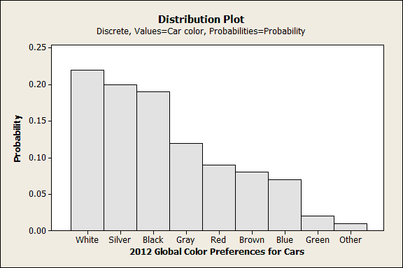
For example, PPG Industries reported the colors of new cars that were purchased in 2012. We can illustrate this using a Probability Distribution Plot (Graph > Probability Distribution Plot). You can use the data in this worksheet if you'd like to try it.
In the Probability Distribution Plots dialog, choose the generic Discrete distribution to supply your own categories and probabilities. You need to enter a column of categories (Car Color) and a column of probabilities (Probability).
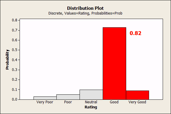
Ordinal Categories
Ordinal categories have a natural order. Values are ranked, but differences do not necessarily represent equal intervals. For example, a rating scale could have the following values: Very Poor, Poor, Neutral, Good, and Very Good. The ordering provides additional information which allows you to do a little more with the data.
For example, in the Probability Distribution Plot below, I had Minitab shade and calculate the cumulative probability (0.82) for all values greater than or equal to Good.
Binary
Binary data can have only two possible values, such as accept or reject. With binary data, you only know whether an event happened, but not the magnitude of the event.
You can use several distributions with binary data. The choice depends on your goal. In these examples, be sure to notice the important differences between the probabilities for each discrete value (each bar in the plots) and the cumulative probabilities (the shaded areas). These examples don't use data in the worksheet.
Binomial distribution
Use the binomial distribution when you are interested in the number of times an event occurs given a specific number of trials. In Minitab, the P Chart and Laney P’ Chart are control charts that use the binomial distribution to determine whether the process is in control.
Suppose you are interested in knowing how likely it is to observe 2 or more defective items in a random sample of 25 items that are selected from a process that has a 2% defect rate.
In the Probability Distribution Plot – View Probability dialog (Graph > Probability Distribution Plot > View Probability), choose the binomial distribution, enter 25 trials, and an event probability of 0.02. Go to the Shaded Area tab and choose X Value, Right Tail, and enter 2.
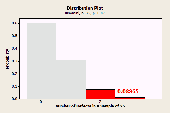
The plot displays the probability for each number of defects in a sample of 25. The probability of exactly zero defects in a sample of 25 is about 0.6, 1 defect is 0.3, etc. Because we asked for a shaded area for 2 or more, Minitab shades that area red and indicates that the cumulative probability of 2 or more defects is 0.08865.
Geometric distribution
Use the geometric distribution when you are interested in the number of consecutive trials necessary to observe the event for the first time.
For example, let’s assume again that the defect rate is 0.02 and we want to model the number of samples we’d have to draw before seeing the first defect. Specifically, we want to determine at what sample size we have a 50% chance of observing a defect.
In the Probability Distribution Plot – View Probability dialog, choose the Geometric distribution and enter an event probability of 0.02. Go to the Shaded Area tab and choose Probability, Left Tail, and enter 0.5.
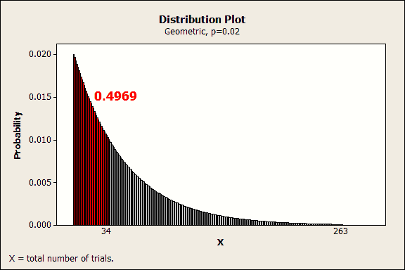
Each bar represents the probability of seeing the first defect on a specific trial. You can hover over a bar to see the probability for a specific trial. For example, the probability of seeing the first defect on exactly the tenth trial is about 0.016.
We’ve asked Minitab to shade the distribution for a cumulative probability of 0.5. The red area indicates that there is a cumulative probability of 0.4969 for observing the first defect within the first 34 trials.
Negative binomial distribution
Use the negative binomial distribution when you are interested in the number of trials necessary to produce the event a specified number of times. For example, this distribution can model the number of windshields produced until you reach 10 defective units.
Assume that the process is stable and has a 0.05 probability of producing a defective windshield. You are interested in the cumulative probability of producing 10 defective windshields in a batch size of 100 windshields.
In the Probability Distribution Plot – View Probability dialog, choose Negative binomial, enter 0.05 for the event probability, and 10 for the number of events need. On the Shaded Area tab, choose X Value, Left Tail, and enter 100.
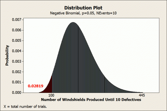
It may be hard to see in the small graph, but there is a bar for each batch size. Each bar represents the probability of exactly 10 defects occurring in a batch of exactly that size. For example, the probability of observing exactly 10 defects in a batch of exactly 75 windshields is slightly less than 0.0004.
We’ve asked Minitab to shade the distribution for 100 units and less. The shaded area in red indicates that there is a cumulative probability of 0.02819 of producing 10 defects within the first 100 units.
Closing Thoughts
I hope this gives you a better grasp of some of the key discrete distributions and how to use them. In the next post, I’ll show you how to determine whether your data follow a specific discrete distribution.