In my last post we looked at different discrete distributions and how you can use them. This time, I’ll show you how to determine whether your data follow a specific discrete distribution. (Read here to see how to identify the distribution of your continuous data.)
Before we start testing discrete distributions, we need to distinguish between two general cases. In some cases, it is more important to:
- Check the assumptions (binary data)
- Perform a goodness-of-fit test
Checking Assumptions for Distributions that Use Binary Data
For the distributions of binary data, you primarily need to determine whether your data satisfy the assumptions for that distribution. If you satisfy the assumptions, you can use the distribution to model the process.
As an example, we’ll walk through the assumptions for the binomial distribution. The binomial distribution has the following four assumptions:
- Each trial has one of two outcomes: This can be pass or fail, accept or reject, etc.
- Each trial is independent: A trial in an experiment is independent if the likelihood of each possible outcome does not change from trial to trial. For example, if you toss a coin 50 times, each coin toss is an independent trial, because the outcome of one toss (heads or tails) does not affect the likelihood of getting a heads or tails on the next toss.
- The probability of an event is the same for each trial: The probability doesn’t change over time. Sometimes you can make this assumption because of the physical properties that are involved, such as flipping a coin. Other times, you may want to use the P Chart to confirm this assumption. If the P Chart is in control, the probability is constant.
- The number of trials is fixed: This assumption reflects your goal that you want to model how frequently the event occurs over a constant number of trials.
Generally, determining whether your data satisfy these assumptions relies on a close understanding of the process, data collection procedure, and your goals for the data. If you satisfy all of these assumptions, you can safely use the binomial distribution.
Besides the binomial distribution, there are three other distributions in Minitab statistical software that use binary data. They each have somewhat different assumptions than those listed for the binomial distribution.
| Distribution |
Key difference from binomial |
| Negative binomial |
You want to model the number of trials to produce a fixed number of events |
| Geometric |
You want to model the number of trials to produce the first event |
| Hypergeometric |
The probability changes overtime as you draw a sample from a small population without replacement |
In short, if you have binary data, the choice of which binary distribution you should use depends on the population, the stability of the proportion, and what you want to do with the data. After you confirm the assumptions, you generally don’t need to perform a goodness-of-fit test.
Performing a Goodness-of-Fit Test
If you suspect that your data follow the Poisson distribution or a distribution based on categorical data, you should perform a goodness-of-fit test to determine whether your data follow a specific distribution. These tests compare the observed values to theoretical values to determine whether there is a significant difference. We’ll walk through some examples so you can see how easy it is to perform these tests. You can get the data here.
Poisson distribution
If you want to determine whether your data follow the Poisson distribution, Minitab has a test specifically for this distribution. To recap, the Poisson distribution describes a count of a characteristic (e.g., defects) over a constant observation space, such as the number of scratches on a windshield.
Accident count example
An insurance agent wants to monitor the number of accidents per month at a particular intersection. The agent records the number of accidents in the worksheet like this:

Each cell in the worksheet represents the number of accidents over one month.
In Minitab, use the Goodness-of-Fit Test for Poisson in the Stat > Basic Statistics menu. In the dialog box, in Variable, enter Accidents, and click OK.
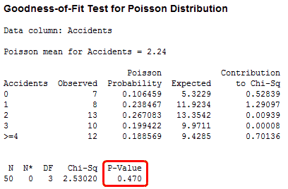
The p-value is 0.470, which is greater than the common alpha level of 0.05. This result suggests that these data follow the Poisson distribution and can be used with analyses that make this assumption. These analyses include the 1- and 2-sample Poisson rate analyses, the U Chart, and the Laney U’ Chart.
Categorical distributions
You can test distributions that are based on categorical data in Minitab using the Chi-Square Goodness-of-Fit Test, which is similar to the Poisson Goodness-of-Fit Test. However, because Minitab doesn’t know the distribution, you need to specify the test proportions yourself.
Car color example
We’ll run through an example using the proportions of car colors from my previous blog. In this example, the global proportions reported by PPG Industries are real, while the observations we “gathered” are for illustrative purposes only.
Suppose we want to determine whether the distribution of car colors in our state match the global distribution. To do this, we have observers around the state record the colors of cars that were manufactured in 2012 and included in a random sample. We tally up the colors and enter the global proportions in the worksheet like this:
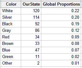
The values in the OurState column represent the tally for each color in our sample. The global proportions are the values reported by PPG Industries.
In Minitab, go to Stat > Tables > Chi-Square Goodness-of-Fit Test (One Variable). In this dialog, enter OurState in Observed counts; enter Color in Category names; and, under Test, choose Specific proportions and enter Global Proportions. Click OK.
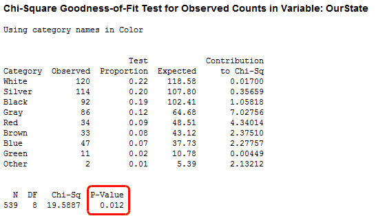
Minitab checks to see if the observed counts differ from the global distribution. A low p-value suggests that your data do not follow that distribution. In this case, the p-value is 0.012, which suggests that the distribution of car colors in our state does not match the global distribution. You can compare the Observed and Expected columns in the table to see where the largest differences occur, or look at the default graphs below.
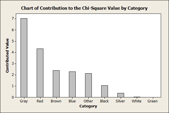
The graph above shows which colors statistically contribute the most to the significant difference. Gray and red contribute the most, more than half. However, the graph doesn’t show whether the observations are higher or lower than the expected value. The next graph addresses that.
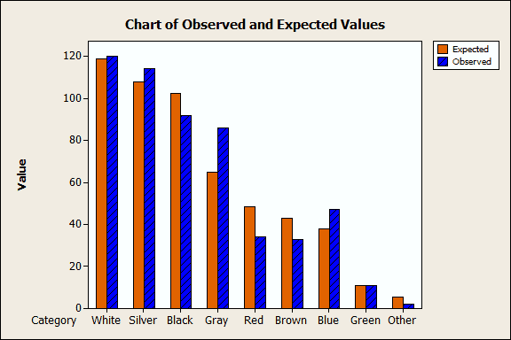
Look at the "Gray" and "Red" bars in the graph above. The observed count of gray cars is greater than the expected count. Conversely, the observed count of red cars is less than the expected count.
Closing Thoughts
We’ve covered a variety of discrete data and how you should test it before you use a discrete distribution to model it. In order to determine how to proceed with your discrete data, you first need to determine what type it is, or suspect that it is. To quickly summarize:
- Binary data: check the assumptions
- Poisson data: use the Poisson Goodness-of-Fit Test
- Other categorical data: use the Chi-Square Goodness-of-Fit Test and specify the test proportions


