


Here at the lightsaber factory, we've completed several steps in doing a capability analysis:
- We made sure our data was collected and entered correctly in Minitab
- We identified the distribution of the data
- We made sure all of our assumptions checked out
We’re getting close to our deadline, and it’s finally time to carry out our Capability Analysis and see if we are manufacturing our lightsabers to the correct specifications as set forth by the Jedi Temple.
First, let’s go to Stat > Quality Tools > Capability Analysis > Normal. (If you want to play along and you don't already have it, get the free 30-day-trial of our statistical software.) Fill out the dialog as follows:
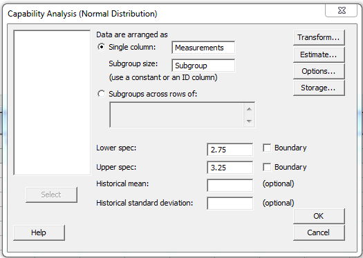
In addition, click on the "Options" button, and add a Target of 3. Once we have this, we can click OK and Minitab will perform our Capability Analysis.
Looking at the results, there are a lot of numbers and a lot of abbreviations. It can get confusing, so let’s look a little deeper at each piece of output.
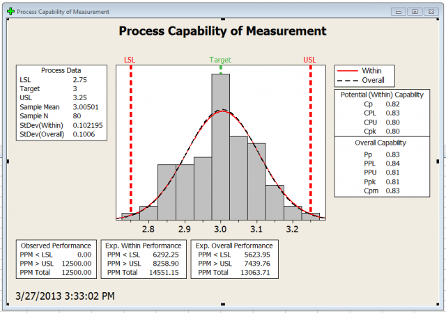
First, at the top left you can see the Process Data box. This is just an overview of some descriptive statistics. It shows our lower spec limit (LSL), upper spec limit (USL), and Target values, as well as the mean, number of observations, and standard deviations that are calculated from our data.
You'll notice there are two different standard deviations that get calculated. The first is the overall standard deviation. This is exactly what it sounds like, the standard deviation among all of your points. The second is the within-subgroup standard deviation. This is the standard deviation within your subgroups.
Now, we can look at the Potential, or within, Capability on the right-hand side of the graph. These are Capability indices that are calculated using your within-subgroup variation. Below that overall Capability, which is associated with the overall standard deviation. The statistics are similar for both. Cp and Pp compares the process spread to the specification spread. The process spread is your standard deviation times a multiplier. The multiplier is usually 6, which would put 99.74% of the observations within +/- 3 sigma of the mean. The specification spread is just your USL-LSL. In this case, our Pp is 0.83 and our Cp is 0.82.
It looks like our process needs to be improved to meet the requirements of the temple.
The PPL, CPL, PPU, and CPU respectively, relate the process spread to the single-sided specification spread. This is beneficial because it takes into account your process spread as well as your process center. However, the drawback is that they only measure from your process center to one side of your process, either upper or lower. You could fit well within the upper spec, but be way off base on the lower spec. This is why we have Cpk and Ppk.
Ppk and Cpk then take the minimum of your PPL, PPU, or CPL, CPU respectively. This gives us a nice number to look at which takes into account both specification limits as well as your spread. In general (though not necessarily always), this is the number that most people are looking for. The difference between Cpk and Ppk is that Cpk is sometimes referred to as the "potential capability" because it represents the potential your process has at producing parts within spec, presuming there is no variation between subgroups over time. Ppk, however, factors in that subgroup variation, so it gives an indication of where you actually are at this moment in time.
In other words, Cpk is where you can be, and Ppk is where you are. It is important to look at both.
In our case, our Cpk is 0.80, and our Ppk is 0.81. The Jedi Temple uses standard AIAG guidelines, which means we want our Capability indexes greater than 1.33. It is clear we’ve fallen short.
We’ve now carried out our analysis, and we’ve unfortunately come to the conclusion that we are not manufacturing the lightsabers to correct specifications. We’re going to need to consider our process and see what changes we can make to improve. We’ll leave those recommendations up to the Jedi council.