


Bailiff: All Rise. The Honorable Judge Lynn E. R. Peramutter presiding.
Judge: Please be seated. Bailiff, please read the charges.
Bailiff: Your honor, this is the case of the State vs. Lionel Loosefit. The defendant is charged with creating a model that violated the legal requirements for regression. The infractions include:
- Producing grossly nonnormal errors
- Producing errors that lack independence
- Exhibiting nonconstant variance
- Violating the linearity assumption
Judge: Thank you, bailiff. Let’s hear the opening statement by the prosecutor.
Prosecutor: Your honor, ladies and gentlemen of the jury. We’re here today to try the defendant, Mr. Loosefit, on gross statistical misconduct when performing a regression analysis. You heard the bailiff read the charges—not one, but four blatant violations of the critical assumptions for this analysis. Yet, despite being fully aware of the egregious nature of these heinous infractions, the defendant knowingly and willfully used his model, in public, to estimate response values, violating the basic tenets of statistical decency.
[Alarmed murmurs and sudden gasps in the courtroom.]
Judge: (rapping gavel) Order!! How does the defendant plead?
Defense Lawyer: My client pleads “not guilty” to all four charges, your honor.
Judge: (to prosecutor) Counsel, proceed.
Prosecutor: Your honor, these are serious offenses. Because the statistical penal codes are a bit murky, and because our court stenographer is a part-time Minitab blogger who types using only one finger, I’d like to ask the court’s permission to address each charge one blog post at a time.
Judge: Granted.
The Prosecution's Case: Errors of a Highly Nonnormal Nature
Prosecutor: Ladies and gentlemen, today let us examine the charge that that the errors in the defendant’s model lack normality. I’d like to start by calling our expert witness to the stand, Dr. Minnie Tabber, world-renowned statistician.
[Dr. Tabber approaches the stand and places right hand on a thick, leather-bound volume of the cumulative probabilities of the standard normal distribution.]
Bailiff: Do you swear to tell the statistical truth, the whole statistical truth, so help me Ronald Fisher?
Dr. Tabber: I do.
Bailiff: Please take a seat in the witness stand.
Prosecutor: Dr. Tabber, please explain your area of expertise.
Dr. Tabber: My specialty is statistics. My passion is Quality. Data. Analysis.
Prosecutor: And could you briefly explain to the court the requirement of normally distributed errors in a regression model?
Dr. Tabber: Certainly. The errors in any model are just the differences between the actual observations in your data and the expected values predicted by your model. No model is perfect. You expect errors—but you want the errors (which are also called residuals) to be reasonably normal.
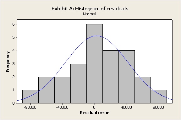
Prosecutor: Your honor, I’d like to introduce Exhibit A, a normal histogram of the residuals from a regression model:
Prosecutor: Could you explain what we’re seeing here, Dr. Tabber?
Dr. Tabber: Sure. This is a histogram of the errors from a model. The horizontal scale shows the difference between the data observation and the value predicted by the model. It tells you the size of the errors. Notice that most errors are at or close to 0—that’s what you want to see. It means most of the data don’t deviate much from the values predicted by the regression model. As the size of the errors become larger in either direction, there are fewer and fewer of them, and they’re spread roughly evenly on both sides.
Prosecutor: In other words, the distribution of the errors in Exhibit A is fairly normal.
Dr. Tabber: Yes. The residuals don’t have to perfectly follow the bell curve indicated by the blue line. But basically you want the highest bar to be close to 0, and the bars on each side to be progressively smaller—showing no strong tendency of the model to overestimate or underestimate values.
Prosecutor: Your honor, I’d like to introduce Exhibit B, the histogram of the residuals from the defendant’s model.
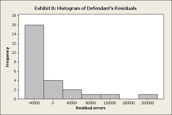
Prosecutor: Dr. Tabber, would anyone in their right mind call these errors normal?
Dr. Tabber: It would take quite a few martinis to make that look like a bell curve. That model appears to be quite inconsistent in how it overestimates and underestimates response values.
Prosecutor: Of course. Even a kindergartner can see the errors are extremely skewed to the right. Where’s the left tail? Why, it doesn’t exist! Did somebody steal the left tail from the defendant’s residuals? Perhaps it's been swiped by a wild, merry gang of number crunchers, who are using it to play a game of pin the tail on the histogram!
[Laughter in the courtroom].
Judge: (rapping gavel) Order!!
Prosecutor: No further questions your honor.
The Cross Examination: Do Bins Make the Bells?
Judge (to defense attorney): You may cross-examine the witness.
Defense Attorney: Dr. Tabber, you mentioned that the residuals don’t have to be perfectly normal, is that correct?
Dr. Tabber: Yes, that’s correct. They should be roughly normal to satisfy the requirements for regression.
Defense Attorney: Dr. Tabber, have you ever heard the famous quotation: “The only normal people are the ones you don’t know very well”?
Dr. Tabber: That sounds vaguely familiar…
Defense Attorney: What, really, is “normal”? After all, we all make errors, don’t we? Like taking a wrong turn...getting someone’s name wrong… brushing your teeth with shaving cream… forgetting to file taxes for several years in a row...
[Judge raises an eyebrow.]
Defense Attorney: Dr. Tabber, would you consider it normal to sing to yourself while driving alone in your car?
Dr. Tabber: Personally, I don’t do that—but yes, I’d consider that normal behavior.
Defense Attorney: Of course. What about talking to yourself out loud while driving alone in your car? And I don’t mean using a phone.
Dr. Tabber: Well, uh, I’m not sure…
Defense Attorney: Of course, you’ve never done anything abnormal like that, have you? All of your errors are perfectly normal, aren’t they?
Prosecutor: Objection, your honor! This is irrelevant—the issue here is the normality of the defendant’s residuals, not the normality of a statistician.
Judge: Sustained. Counsel, keep your questions addressed to the residuals.
Defense Attorney: Your honor, I’d like to introduce Exhibit C, another histogram of residuals.
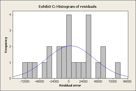
Defense Attorney: Dr. Tabber, would you be satisfied that the residuals in Exhibit C are normally distributed?
Dr. Tabber: I’d have some misgivings about that.
Defense Attorney: What concerns you?
Dr. Tabber: Well, the data appear to be bimodal—with two centers. And the high frequency of errors from 26000 to 38000 is troubling.
Defense Attorney: Troubling, yes. Indeed.
[Pauses, then turns to jury box.]
Defense Attorney: But you know what’s really troubling, Dr. Tabber? These are the exact same residuals as in Exhibit A—which gave us that lovely, beautiful bell curve. The only difference is that this histogram uses different intervals to define the bins. It's the same data in different cans.
[Murmurs in the courtroom]
Defense Attorney: Suddenly, we’ve gone from “normal” to “troubling”… just by changing the number of bins on the graph. Yet the evidence—the errors—haven't changed. Dr. Tabber, might we say then, that normality, like beauty, can be very much in the eye of the beholder?
Dr. Tabber: Well, that might be true in certain instances, but—
Defense Attorney: Thank you. No further questions, your honor.
[Spectators begin nodding to one another.]
The Reexamination: Putting Evidence to the Test
Prosecutor: Your honor, I’d like to briefly re-examine the witness.
Judge (yawning): Keep it short. We’ve all got other work to do. And I’ll remind you our stenographer is typing with his pinky finger.
Prosecutor: Dr. Tabber, are histograms always definitive indicators of normality?
Dr. Tabber: Histograms are pretty accurate with large data sets, but with small data sets the binning intervals on the graph can greatly affect its appearance, as we have just seen.
Prosecutor: So is there nothing we can do? Must we just wring our hands and assume no one can say whether data is normal or nonnormal? Do we assume that we can’t separate up from down? Or that the planet is spinning senselessly in a chaotic cosmos devoid of meaning, with all distributions being relative and arbitrary?
Dr. Tabber: Most definitely not. Minitab has other tools to assess normality, such as the probability plot.
Prosecutor: Your honor, I’d like to introduce Exhibit D, a normal probability plot of the defendant's residuals.
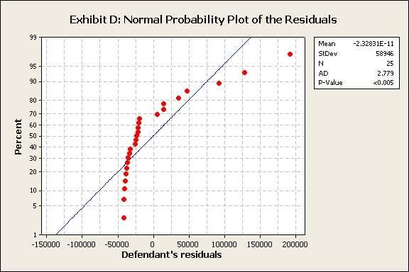
Prosecutor: Dr. Tabber, there are lots of points, lines, and numbers here—can you translate for us?
Dr. Tabber: The blue line shows the expected percentiles for the given distribution—in this case, the normal distribution. The red points show the actual values in the data set. Basically, you want the red points to fall along the blue line—that means your data fits the given distribution.
Prosecutor: So you want those big red dots to appear like a long, skinny caterpillar on the blue branch?
Dr. Tabber: I guess you could say that…
Prosecutor: Not like a snake that’s looped around the branch, its tail dangling toward the ground, its head in the air, slithering toward its innocent prey…
[Horrified gasps in the courtroom]
Defense Attorney: Objection, your honor!!
Judge: Sustained.
Prosecutor: So in this case, does the probability plot indicate that the errors in the defendant’s model are roughly normally distributed?
Dr. Tabber: Not at all. And neither do the results for the Anderson-Darling (AD) normality test.
Prosecutor: Where do we see those test results?
Dr. Tabber: They’re shown by the p-value in the graph legend. If the p-value is less than the alpha level of 0.05, we reject the assumption that the data follow the normal distribution.
Prosecutor: How sure are you about these results?
Dr. Tabber: Well, the p-value is < 0.005, so the chance of obtaining such a result, purely by chance, if the data were actually normal, is less than 1 in 200.
Prosecutor: So there’s no doubt in your mind these data deviate significantly from a normal distribution?
Dr. Tabber: Based on the histogram, the probability plot, and the Anderson-Darling (AD) test for normality, there’s no way these residuals could be called normal.
Prosecutor: Your honor, ladies and gentlemen of the jury. As we’ve clearly shown, the errors in the defendant’s regression model are not normal. In fact, these model errors can only be called shockingly deviant, flying in the face of all decent standards of normality!
[Pandemonium breaks loose in the courtroom.]
Spectator 1: “Lock him up!”
Spectator 2: “Throw the textbook at him!”
Spectator 3: “Take away his model!”
Spectator 4: “Make him eat his rotten coefficients!!”
Judge: (slamming gavel) Order! Order! This court is adjourned. We’ll take a 2-week recess before addressing the other charges.
Read Part 2 of the trial transcript
Illustration: The Jury, by John Morgan (1861) public domain image.