


For one reason or another, the response variable in a regression analysis might not satisfy one or more of the assumptions of ordinary least squares regression. The residuals might follow a skewed distribution or the residuals might curve as the predictions increase. A common solution when problems arise with the assumptions of ordinary least squares regression is to transform the response variable so that the data do meet the assumptions. Minitab makes the transformation simple by including the Box-Cox button. Try it for yourself and see how easy it is!
The government in Queensland, Australia shares data about the number of complaints about its public transportation service.
I’m going to use the data set titled “Patronage and Complaints.” I’ll analyze the data a bit more thoroughly later, but for now I want to focus on the transformation. The variables in this data set are the date, the number of passenger trips, the number of complaints about a frequent rider card, and the number of other customer complaints. I'm using the range of the data from the week ending July 7th, 2012 to December 22nd 2013. I’m excluding the data for the last week of 2012 because ridership is so much lower compared to other weeks.
If you want to follow along, you can download my Minitab data sheet. If you don't already have it, you can download Minitab and use it free for 30 days.
Let’s say that we want to use the number of complaints about the frequent rider card as the response variable. The number of other complaints and the date are the predictors. The resulting normal probability plot of the residuals shows an s-curve.
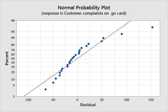
Because we see this pattern, we’d like to go ahead and do the Box-Cox transformation. Try this:
- Choose Stat > Regression > Regression > Fit Regression Model.
- In Responses, enter the column with the number of complaints on the go card.
- In Continuous Predictors, enter the columns that contain the other customer complaints and the date.
- Click Options.
- Under Box-Cox transformation, select Optimal λ.
- Click OK.
- Click Graphs.
- Select Individual plots and check Normal plot of residuals.
- Click OK twice.
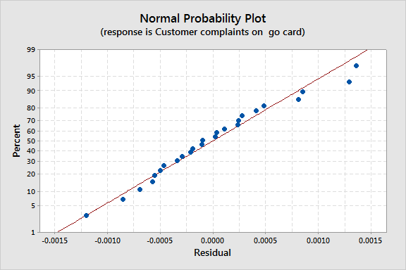
The probability plot that results is more linear, although it still shows outlying observations where the number of complaints in the response are very high or very low relative to the number of other complaints. You'll still want to check the other regression assumptions, such as homoscedasticity.
So there it is, everything that you need to know to use a Box-Cox transformation on the response in a regression model. Easy, right? Ready for some more? Check out more of the analysis steps that Minitab makes easy.
The image of the Translink vending machine is by Brad Wood and is licensed for reuse under this Creative Commons License.