


When performing a design of experiments (DOE), some factor levels may be very difficult to change—for example, temperature changes for a furnace. Under these circumstances, completely randomizing the order in which tests are run becomes almost impossible.To minimize the number of factor level changes for a Hard-to-Change (HTC) factor, a split-plot design is required.
Why Do We Want to Randomize a Designed Experiment?
Randomization means that the experimental tests are run in a random order specified by Minitab, and that factor level changes occur randomly. Randomization in a DOE is desirable, because it helps ensure that factor estimates are not biased by long-term drifts during the experiments.
Suppose that, due to environmental conditions, a gradual change in temperature takes place during the tests. This gradual change may affect factor effect estimates. If most of the tests are performed at the lower setting for a particular factor at the beginning of the experiment, and then most of the tests at the end use the upper settings of this factor, then temperature effect and the drift will be erroneously attributed to this factor, leading to biases and wrong conclusions.
That's why complete randomization in a DOE is desirable. When you can randomize, a drift in environmental conditions will not have a systematic effect on some factor estimates. There will certainly be a random impact, but not a systematic one. But when HTC factors need to be studied, randomization is not always possible.
Enter the split-plot design.
What Is a Split-Plot design
The first designs of experiments were agricultural experiments at the beginning of the 20th century. Think about a large field in which experiments need to be performed to test different types of plant varieties, fertilizers, soil treatments, etc.
This experimental field may be divided into plots, and different treatments will be allocated to these plots. If the number of level changes needs to be minimized for a specific HTC factor, large plots of the field will be used. These are referred to as whole plots.
For an Easy-to-Change (ETC) factor, smaller plots may be used. We create these sub-plots by subdividing the whole plots into the smaller subplots.
In the presence of spatial variability in the experimental field, we can expect soil variations to be smaller when subplots are located close to one another, whereas we would expect soil variations to be much larger between whole plots since they are located further from one another.
In a manufacturing context, whole plots represent long-term variations and sub plots represent short-term variations. To estimate long-term variations, whole plots need to be replicated.
To minimize complex modifications of settings, the levels of HTC factors are never changed within a whole plot and all the runs within a whole plot are performed together, in the same period of time.
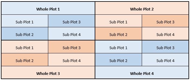
The field above has been divided into four whole plots, and the whole plots have then been subdivided into subplots.
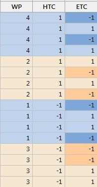
A split plot design array as displayed in Minitab Statistical Software appears below, with different colors for whole plots and subplots (see below). In the HTC column the 1 or -1 settings are changed much less often than in the ETC column:
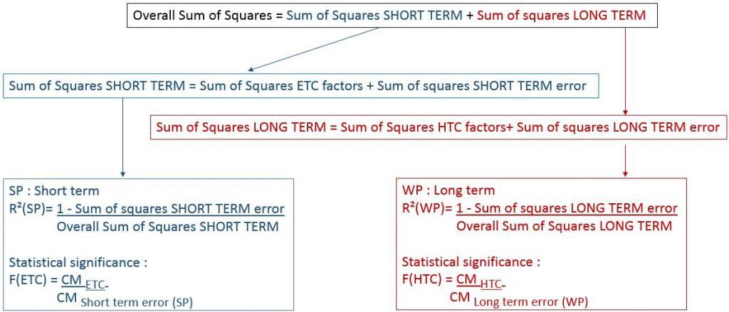
There are two main sources of variations to be considered in a split plot design: short-term variation (between subplots: SP) and long-term variation (between whole plots: WP). Hard-to-Change (WP) factors are affected by long term variability whereas Easy-to-Change (SP) factors are affected by short term variability.
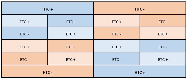
- HTC + : treatment at the upper setting for the Hard to change factor
- HTC - : treatment at the lower setting for the Hard to change factor
- ETC + : treatment at the upper setting for the Easy to change factor
- ETC - : treatment at the lower setting for the Easy to change factor
To determine whether a factor is significant or not (according to the F test), the effects of ETC factors will be compared to the short-term error term (SP) only, whereas the effects of HTC factors will be compared to the long term error term (WP) only.
Also, two R² estimates are displayed in a split plot design analysis: a short term R² and a long term R².
To compute the short term R² value (SP), the amount of variability which is explained by short-term, Easy-to-Change (SP) factors is compared to the short-term overall (subplot sum of squares) variability.
To estimate the long-term R² value (WP), the amount of variability explained by long term Hard-to-Change (WP) factors will be compared to the long term overall (WP sum of squares) variability only.
Conclusion
In a split plot design, two error terms need to be considered (short term and long term) separately, and two R² values need to be computed (short term and long term). The analysis may look more complex, but that makes the interpretation of the DOE results a lot more realistic.