


In hypothesis testing, we use data from a sample to draw conclusions about a population. First, we make an assumption called the null hypothesis (denoted by H0). As soon as you make a null hypothesis, you also define an alternative hypothesis (Ha), which is the opposite of the null. Sample data will be used to determine whether H0 can be rejected. If it is rejected, the statistical conclusion is that the alternative hypothesis Ha is true.
Keep in Mind the Power of the Test, or the Probability of Rejecting the Null Hypothesis When the Null Is Not True
It could be interpreted as the “ability of the test to reject the null when it is supposed to be rejected”. If the null is not true, it makes sense to have high probability to reject the null hypothesis. Power is related to the Type 2 error (power = 1 -Type 2 error), see the table below. The Type 2 error is the probability of not rejecting the null when the alternative is true. So, guaranteeing a high enough power guarantees a low or “acceptable” Type 2 error. A popular way to ensure the test has enough power is by collecting enough data because the calculation of power depends on the sample size, among other things. The larger the sample size, the higher the power. On the other hand, not collecting enough data will yield low power and a high type 2 error.
|
|
Truth |
|
|
Decision of Hypothesis Test |
H0 is True |
Ha is True |
|
Reject H0 |
Type 1 Error, α |
Power (1-β) |
|
Fail to Reject H0 |
Correct |
Type 2 Error, β |
It is important to find an appropriate sample size. Clearly, not collecting enough data leads to a higher Type 2 error. However, collecting “too much” data can increase the Type 1 error because the test will have high power. As a result, the test might detect a very small difference from the hypothesized value, even though that difference may not be of any practical significance, especially in relation to the cost of sampling. The calculation of the power of a test should be based on practical significance.
Minitab Statistical Software Has Functionality for Calculating the Power for Many Different Statistical Tests
In the following example, an analyst does a power and sample size analysis in Minitab for the 1 proportion test and the 1 sample t test.
Sample size for 1 proportion test
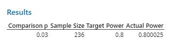
Consider a manufacturing process that classifies products as good or bad is operating with 1% defective. If the percent of defectives increases to 3%, this will have serious cost implications to the organization. They are required to determine an appropriate sample size such that: the type I error rate will be 0.05, and for the test to have a power of 0.80 to detect an increase in the defectives from 1% to 3% or above.
Because the analyst is interested in studying the percent defective, they will use a 1 proportion test. The null and alternative hypotheses are:
Ho: P = 0.01
Ha: P > 0.01
where P is the true proportion defective.
To find out how many data points are needed to achieve a power of at least .8, the analyst does a power and sample size analysis for a 1 proportion test in Minitab.
Sample Size for 1 sample t test
Classifying a product as good or bad is simple but suffers from information loss. Consider good as anything between 5 and 10. Suppose we have 2 units measured as 4.9 and 10.01 and thus classified as bad. Suppose we have another 2 units measured as 2.3 and 14.1 and thus classified as bad. Notice if simply say good and bad, these two scenarios are the same. Thus, if measuring a product quality characteristic is possible and practical, then the analyst should record the actual value of the quality characteristic and use the data as it is recorded – no need to convert to good and bad. A 1 sample t test can be used to test whether the mean of the population is on target. If the average from the sample data is close to a “target”, then the process is probably doing well. But if the average is not close to the target, defective products could be produced.
For example, assume that the product characteristic is the diameter of a hole with a specific target. Instead of inspecting 236 products to determine if the hole meets specifications, the analyst could measure the diameter of the hole on each product and compare the average to the target using a 1 sample t test.
To find out how many data points are needed to detect a one sigma shift in the process mean with at least 80% power, the analyst does a power and sample size analysis for a 1 sample t test in Minitab.
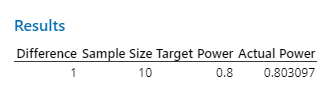
The calculated sample size is only 10. This means that if the analyst wants to determine if the average deviates from the target by more than 1 sigma, they need to inspect 10 units for the 1 sample t test to have at least 80% power.
Why such a big difference?
Hypothesis tests for attribute data requires a large sample size due to fact that no detailed information is captured when collecting the data. On the other hand, hypothesis tests for continuous data require a smaller sample size because the detailed information about the product is captured and used. This concept applies to more than just power. Attribute data require larger sample sizes for confidence intervals, attribute agreement analysis, control charts, and capability analysis.
In conclusion, it is important to conduct a hypothesis test with enough power to give a reasonable chance to detect a difference. Power is directly related to the sample size. Minitab has functionality for calculating power for many different hypothesis tests including design of experiment.