


by Kevin Clay, guest blogger
In transactional or service processes, we often deal with lead-time data, and usually that data does not follow the normal distribution.
Consider a Lean Six Sigma project to reduce the lead time required to install an information technology solution at a customer site. It should take no more than 30 days—working 10 hours per day Monday–Friday—to complete, test and certify the installation. Following the standard process, the target lead time should be around 24 days.
Twenty-four days may be the target, but we know customer satisfaction increases as we complete the installation faster. We need to understand our baseline capability to meet that demand, so we can perform a capability analysis.
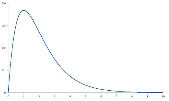
We know our data should fit a non-normal (positively skewed) distribution. It should resemble a ski-slope like the picture below:
In this post, I will cover five simple steps to understand the capability of a non-normal process to meet customer demands.
1. Collect data
First we must gather data from the process. In this scenario, we are collecting sample data. We pull 100 samples that cover the full range of variation that occurs in the process.
In this case the full range of variation comes from three installation teams. We will take at least 30 data points from each team.
2. Identify the Shape of the Distribution
We know that the data should fit a non-normal distribution. As Lean Six Sigma practitioners, we must prove our assumption with data. In this case, we can conduct a normality test to prove non-normality.
We are using Minitab as the statistical analysis tool, and our data are available in this worksheet. (If you want to follow along and don't already have it, download the free Minitab trial.)
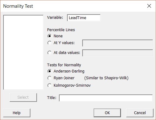
From the menu, select “Normality Test” found under “Stat > Basic Statistics > Normality Test …”
Populate the “Variable:” field with LeadTime, and click OK as shown:
You should get the following Probability Plot:
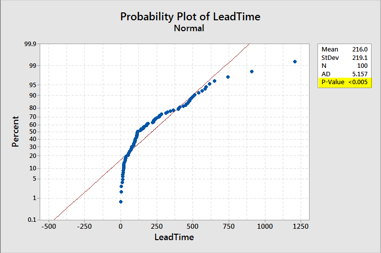
Since the P-value (outlined in yellow in the above picture) is less than .05, we assume with 95% confidence the data fits a non-normal distribution.
3. Verify Stability
In a Lean Six Sigma project, we might find the answer to our problem anywhere on the DMAIC roadmap. Belts need to learn to look for the signals all throughout the project.
In this case, signals can come from instability in our process. They show up as red dots on a control chart.
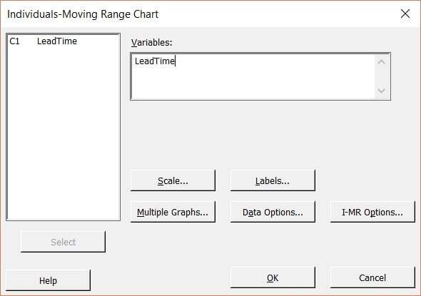
To see if this lead time process is stable, we will run an I-MR Chart. In Minitab, select Stat > Control Charts > Variables Charts for Individuals > I-MR…”
Populate “Varibles:” with “LeadTime” in the dialog as shown below:
Press OK, and you'll get the following “I-MR Chart of LeadTime”:
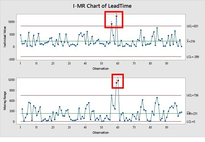
The I-MR Chart shows two signal of instability (shown as red dots) on both the Individual Chart on the top of the graph, and the Moving Range Chart on the bottom.
These data points indicate abnormal variation, and their cause should be investigated. These signals could offer great insight into the problem you are trying to solve. Once identified and resolved the causes of these points, you can take additional data or remove the points from the data set.
In this scenario, we will leave the two points in the data set (we will not remove the two points)
4. What Non-Normal Distribution Does the Data Best Fit?
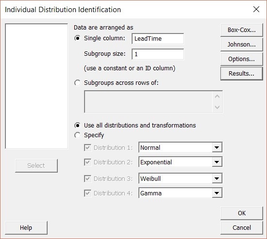
There are several non-normal data distributions that the data could fit, so we will use a tool in Minitab to show us which distribution fits the data best. Open the “Individual Distribution Identification” dialog by going to Stat > Quality Tools > Individual Distribution Identification…
Populate “Single column:” and Subgroup size:” as follows:
Minitab will output the four graphs shown below. Each graph includes four different distributions:
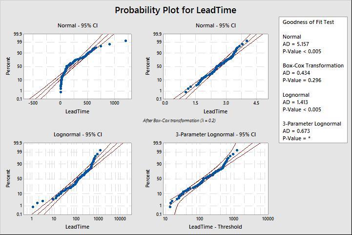
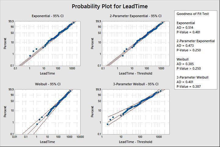
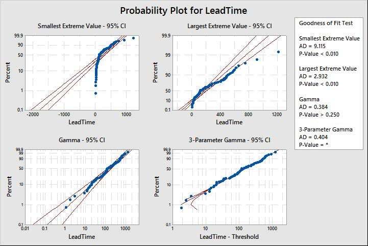
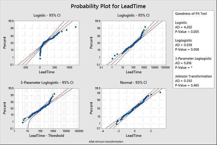
Pick a distribution or transformation with a p-value above your chosen alpha level (typically 0.05). Note, as general rule-of-thumb, don’t consider a transformation unless no distribution fits. In this scenario, we choose the exponential distribution.
5. What Is the Process Capability?
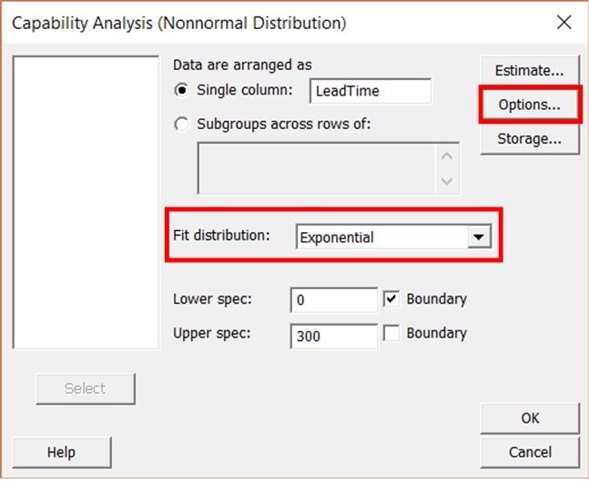
Now that we know the distribution that best fits these data, we can perform the non-normal capability analysis. In Minitab, select Stat > Quality Tools > Capability Analysis > Nonnormal…
Populate the “Capability Analysis (Nonnormal Distribution)” dialogue box as seen below. Make sure to select “Exponential” next to Fit distribution. Then, Click on “Options”.
Fill in the “Capability Analysis (Non Normal Distribution): Options” dialogue box with the following:
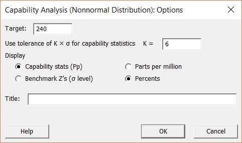
We chose “Percents” over “Parts Per Million” because in this scenario it would take years to produce over one million outputs (or data for each installation time).
OK out of the options and main dialog boxes, and you should get the following “Process Capability Report for LeadTime”:

We interpret the results of a non-normal capability analysis just as we do an analysis done on data with a normal distribution.
Capability is determined by comparing the width of the process variation (VOP) to the width of the specification (VOC).We would like the process spread to be smaller than, and contained within, the specification spread.
That’s clearly not the case with this data.
The Overall Capability index on the right side of the graph depicts how the process is performing relative to the specification limits.
To quickly determine whether the process is capable, compare Ppk with your minimum requirement for the indices. Most quality professionals consider 1.33 to be a minimum requirement for a capable process. A value less than 1 is usually considered unacceptable.
With a Ppk of .23, it seems our IT Installation Groups have work ahead to get their process to meet customer specifications. At least these data offer a clear understanding of how much the process can be improved!
About the Guest Blogger:
Kevin Clay is a Master Black Belt and President and CEO of Six Sigma Development Solutions, Inc., certified as an Accredited Training Organization with the International Association of Six Sigma Certification (IASSC). For more information visit www.sixsigmadsi.com or contact Kevin at 866-922-6566 or kclay@sixsigmadsi.com.