


If you want to use data to predict the impact of different variables, whether it's for business or some personal interest, you need to create a model based on the best information you have at your disposal. In this post and subsequent posts throughout the football season, I'm going to share how I've been developing and applying a model for predicting the outcomes of 4th down decisions in Big 10 games. I hope sharing my experiences will help you, whether the questions you want to answer are about football or business logistics.
Here are some questions I was looking to answer when I began thinking about creating a 4th down calculator. If you have a 1st and 10 at your opponent’s 20-yard line, on average you’ll score more points than if you have the ball at your own 20 yard line. But how many more? And how does that number change as you move to different positions on the field. And what if you’re playing on the road as opposed to playing at home?
If you’re trying to use analytics to determine what the best decision is on 4th down, you need to know how many points you (or your opponent) would be expected to score on the ensuing 1st down. So my first step in creating a Big Ten 4th down calculator was to use Minitab Statistical Software to model a team’s expected points on 1st and 10 from anywhere on the field.
The Data
I went through every Big Ten conference game the last two seasons. For each instance a team had 1st and 10, I recorded the field position and the next score. If your opponent was the next team to score, then the value for the next score was negative. If nobody scored before halftime or the end of the game (depending on which half they were in) the value was 0.
I only included conference games because many non-conference games are one-sided (I’m looking at you, Ohio State vs. Kent State in 2014). I also didn’t include the conference championship game, since I want to account for home field advantage and that game is played at a neutral site. Finally, I did my best to exclude drives that ended prematurely because of halftime and drives in the 4th quarter of blowouts.
I ended up with 5,496 drives over the two seasons. You can get both the raw and summarized data here.
A bar chart can give us a quick glance at what the most common score is.
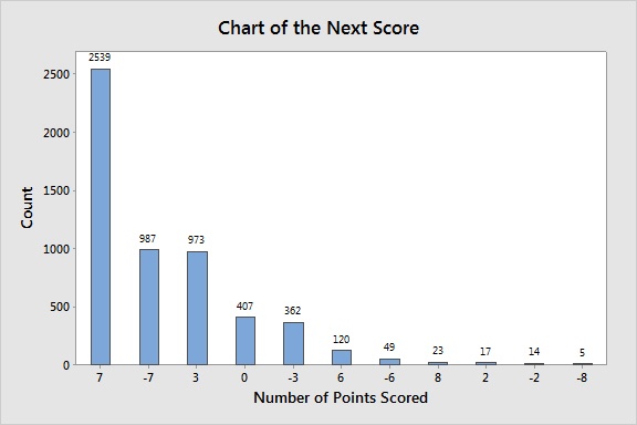
The most common outcome when you have possession of the ball is that you score a touchdown. No revelation there. But surprisingly, it was actually more common for your opponent to get the ball back and score a touchdown than it was for you to kick a field goal. I wouldn’t have expected that.
So now let’s see what happens when we account for the field position and home field advantage.
A Model for Expected Points
I grouped the field position into groups of 5 yards intervals. Then for each group, I took the average of the next score. So first, let’s look at a fitted line plot of the data, without accounting for home field advantage.
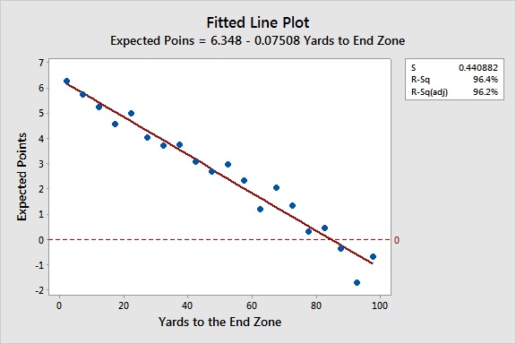
The regression model fits the data very well. The R-squared value indicates that 96.4% of the variation in Expected Points can be explained by the number of yards to the end zone. That’s fantastic! I added a reference line at the point where the expected value is 0. It crosses our regression line at a distance to the end zone of approximately 85 yards. That suggests you have to be inside your own 15 yard line before the team on defense is more likely to be the next team to score.
Now let’s factor in home field advantage. We’ll start by examining a scatterplot that will show the difference in expected points for home and away teams at each yard line group.
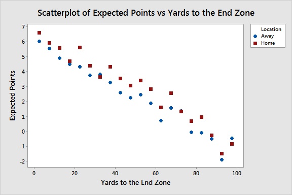
In 17 of the 20 groups, the home team has a higher number of expected points than the away team. And in the 3 cases where the away team is higher, the two values are very close. This gives strong evidence that we need to account for home field advantage. I ran a regression analysis to confirm that we should include that game location in our model.
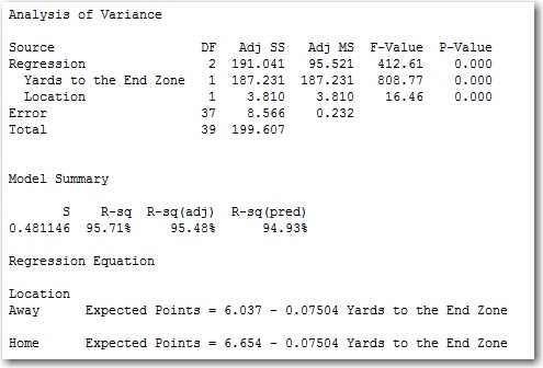
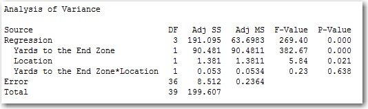
The p-value for location is less than 0.05, and the R-squared value remains very high. I can now use these two equations (one for home games, one for away games) to predict how many points a team with a first down will score from anywhere on the field.
Testing the Interaction Between Home Field Advantage and Yards to the End Zone
There is one last thing I want to look into. Is there an interaction between our two terms? Think about it this way: Say you have 1st and goal inside your opponent’s 10 yard line. You’re so close to the end zone, it seems like it might not matter whether you’re at home or on the road.
Now imagine you have a 1st and 10 inside your own 10 yard line. It seems like a much more daunting task to drive the length of the field on the road with the hostile crowd roaring than it would be with the cheers of a friendly home crowd.
In other words, does the effect of home field advantage increase the further a team is from the end zone? Intuitively, it seems like it should. But we should run a regression analysis to see if the data supports that notion.
The data does not support my intuition. The p-value for the interaction term is much higher than 0.05, indicating that it is not a significant term, and thus that we should not include it in our model. To visualize why, let’s revisit the previous scatterplot, but this time I'll add regression lines to each group.
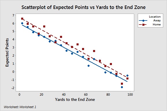
If there were an interaction between our two terms, we would expect the two lines to be close together at small distances to the end zone. Then they should move farther apart as the yards to the end zone increase. But you can see here that the lines are pretty parallel to each other. So we can safely remove the interaction term from our model.
The Final Model
Let’s take a final look at the model created by this regression analysis.
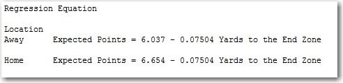
The equations indicate that if you start a drive on the road, you’ll be expected to score approximately 0.6 fewer points than you would if you were playing at home. Because there is no interaction term, the slopes are the same for both equations. The value of -0.075 means that for every yard you move away from the end zone, your expected points decrease by 0.075. So if you decide to punt the football away and get a net of 40 yards (the average in the Big Ten last year), this model indicates you’ll have saved yourself about 3 points on average.
Of course, that 3 points assumes that you turned the ball over on downs. But a third option exists: successfully converting on 4th down.
Will the reward of a successful conversion outweigh the risk of losing those 3 points you would gain by punting? That all depends on the probability of successfully converting on 4th down. And that’s exactly what I'll look at in my next post. Once we can determine the probability of converting on 4th down, we’ll be able to get some data-driven insights into what the correct decision is on 4th down. Stay tuned!