


This past week, the History Channel premiered a new show called the "United Stats of America." No, that's not a typo. It's a show hosted by twin brothers who are both standup comedians and obsessed with statistics. Since I'm also obsessed with statistics (I'm still working on the standup comedy part), I thought I'd check it out to see if I could relate any of their stats to common applications of Minitab Statistical Software.
The show attempts to reveal some of the most interesting and surprising statistics in America. For example, only 8% of teenage boys use soap when they wash their hands. And once a year a meteor the size of a boulder hits the Earth with the descructive force of an atomic bomb (don't worry, 70% of the Earth is covered in water, so odds are you're okay). And on top of that, more Americans are killed by deer each year than snakes. In fact, snakes aren't nearly as dangerous as people think. Your odds of dying from a snake bite are about 1 in 50 million.
And the odds get even safer if you're sober.
Wait, did I just bring booze into this? Yes, yes I did. That's because 40% of people who are bitten by a snake are also legally drunk. So after I erased "Hike the Grand Canyon while drinking" from my bucket list, I thought about this stat and decided that it makes sense. If you're drunk, you're going to be slower and less aware, thus giving the snake a better opportunity to bite you. But this made me wonder, how much slower do you get while intoxicated? That sounded like a great question for Minitab's regression analysis.
NOTE: The following experiment was made up by me for illustrative purposes. I didn't actually do any of this. But you can get my purely illustrative data here if you want to follow along.
On a clear summer morning, I gathered 40 people who knew their 100-yard-dash time. Then I randomly assigned each person a varying amount of alcohol to drink. When they were done, I recorded their Blood Alcohol Content (BAC) and made them run a 100-yard dash. I recorded the difference between the time they ran intoxicated and their regular 100-yard-dash time (Time Difference). Here are the regression results.
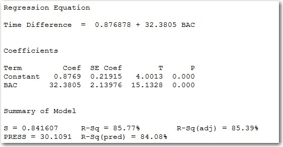
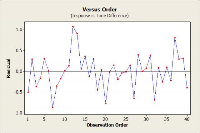
The p-value for BAC is less than 0.05 and our R-Squared value is 85.77%. I'd say we have a pretty good regression model! Of course, we're not done yet. There are assumptions to check! I recorded each runner one at a time and entered their data into Minitab in the order they were tested. So I should make a Residuals vs. Order plot to make sure the order of the runners didn't affect the results.
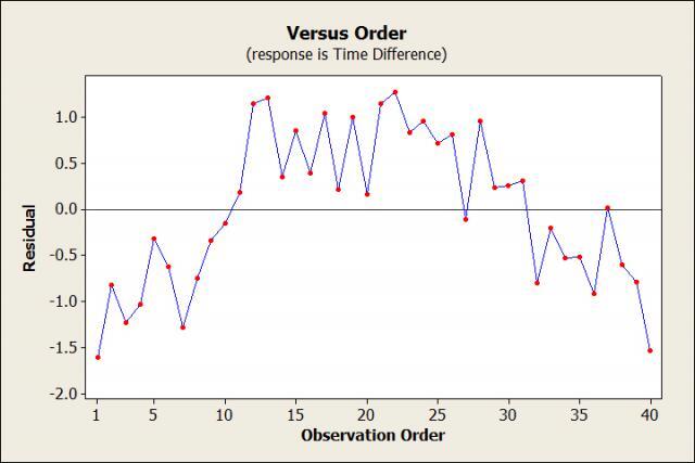
The data should be randomly spread around 0. But wait, this plot doesn't look random at all! Oops, I think I realized what happened. Remember when I said I did the experiment on a clear summer morning? Well, it took awhile to get through all 40 people, so that morning turned into a hot summer afternoon, which then turned into a cool summer evening. Runners that went early or late in the day didn't have to deal with the heat, so their times were faster than expected (negative residual) based on the model. The runners in the middle had to run in the heat, so their times were slower than expected (positive residual). We can plot the residuals versus the variable temperature to test this theory.
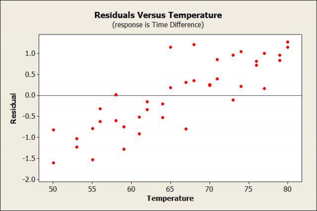
Yep, the residuals definitely increase as temperature increases. So what do I do? Well, one solution would be to redo the experiment somewhere with a constant temperature, like an indoor track. But if I don't have the time for that, I could also add temperature to the regression model. Let's do that and see what happens.
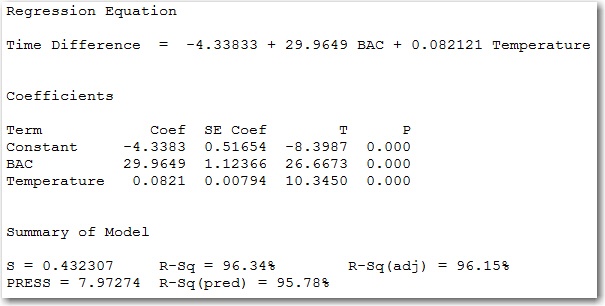
All right, that looks much better! Our R-Squared value increased to 96.34% and our Residuals vs. Order plot looks good: the data are now randomly scattered around 0 with no patterns.
So now that my fake experiment is concluded, I am actually wondering if anybody has ever done a real experiment like this. If not, do I have any volunteers?