Using a sample to estimate the properties of an entire population is common practice in statistics. For example, the mean from a random sample estimates that parameter for an entire population. In linear regression analysis, we’re used to the idea that the regression coefficients are estimates of the true parameters. However, it’s easy to forget that R-squared (R2) is also an estimate. Unfortunately, it has a problem that many other estimates don’t have. R-squared is inherently biased!
In this post, I look at how to obtain an unbiased and reasonably precise estimate of the population R-squared. I also present power and sample size guidelines for regression analysis.
R-squared as a Biased Estimate
R-squared measures the strength of the relationship between the predictors and response. The R-squared in your regression output is a biased estimate based on your sample.
- An unbiased estimate is one that is just as likely to be too high as it is to be too low, and it is correct on average. If you collect a random sample correctly, the sample mean is an unbiased estimate of the population mean.
- A biased estimate is systematically too high or low, and so is the average. It’s like a bathroom scale that always indicates you are heavier than you really are. No one wants that!
R-squared is like the broken bathroom scale: it is deceptively large. Researchers have long recognized that regression’s optimization process takes advantage of chance correlations in the sample data and inflates the R-squared.
This bias is a reason why some practitioners don’t use R-squared at all—it tends to be wrong.
R-squared Shrinkage
What should we do about this bias? Fortunately, there is a solution and you’re probably already familiar with it: adjusted R-squared. I’ve written about using the adjusted R-squared to compare regression models with a different number of terms. Another use is that it is an unbiased estimator of the population R-squared.
Adjusted R-squared does what you’d do with that broken bathroom scale. If you knew the scale was consistently too high, you’d reduce it by an appropriate amount to produce an accurate weight. In statistics this is called shrinkage. (You Seinfeld fans are probably giggling now. Yes, George, we’re talking about shrinkage, but here it’s a good thing!)
We need to shrink the R-squared down so that it is not biased. Adjusted R-squared does this by comparing the sample size to the number of terms in your regression model.
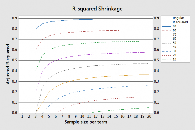
Regression models that have many samples per term produce a better R-squared estimate and require less shrinkage. Conversely, models that have few samples per term require more shrinkage to correct the bias.

The graph shows greater shrinkage when you have a smaller sample size per term and lower R-squared values.
Precision of the Adjusted R-squared Estimate
Now that we have an unbiased estimator, let's take a look at the precision.
Estimates in statistics have both a point estimate and a confidence interval. For example, the sample mean is the point estimate for the population mean. However, the population mean is unlikely to exactly equal the sample mean. A confidence interval provides a range of values that is likely to contain the population mean. Narrower confidence intervals indicate a more precise estimate of the parameter. Larger sample sizes help produce more precise estimates.
All of this is true with the adjusted R-squared as well because it is just another estimate. The adjusted R-squared value is the point estimate, but how precise is it and what’s a good sample size?
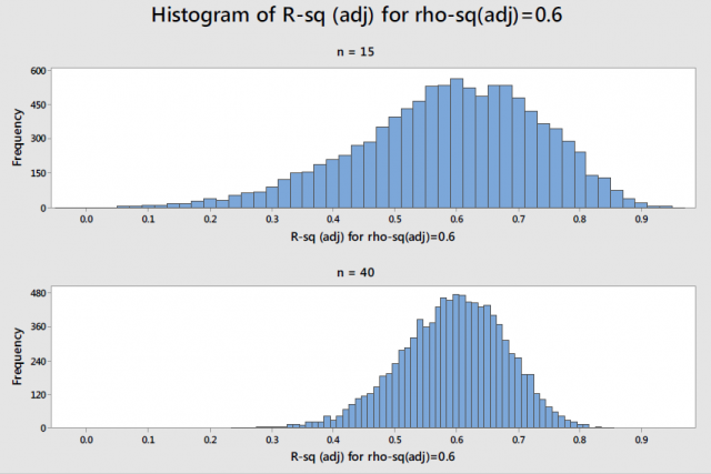
Rob Kelly, a senior statistician at Minitab, was asked to study this issue in order to develop power and sample size guidelines for regression in the Assistant menu. He simulated the distribution of adjusted R-squared values around different population values of R-squared for different sample sizes. This histogram shows the distribution of 10,000 simulated adjusted R-squared values for a true population value of 0.6 (rho-sq (adj)) for a simple regression model.

With 15 observations, the adjusted R-squared varies widely around the population value. Increasing the sample size from 15 to 40 greatly reduces the likely magnitude of the difference. With a sample size of 40 observations for a simple regression model, the margin of error for a 90% confidence interval is +/- 20%. For multiple regression models, the sample size guidelines increase as you add terms to the model.
Power and Sample Size Guidelines for Regression Analysis
These guidelines help ensure that you have sufficient power to detect a relationship and provide a reasonably precise estimate of the strength of that relationship. Specifically, if you follow these guidelines:
- The power of the overall F-test ranges from about 0.8 to 0.9 for a moderately weak relationship (0.25). Stronger relationships yield higher power.
- You can be 90% confident that the adjusted R-squared in your output is within +/- 20% of the true population R-squared value. Stronger relationships (~0.9) produce more precise estimates.
| Terms |
Total sample size |
| 1-3 |
40 |
| 4-6 |
45 |
| 7-8 |
50 |
| 9-11 |
55 |
| 12-14 |
60 |
| 15-18 |
65 |
| 19-21 |
70 |
In closing, if you want to estimate the strength of the relationship in the population, assess the adjusted R-squared and consider the precision of the estimate.
Even when you meet the sample size guidelines for regression, the adjusted R-squared is a rough estimate. If the adjusted R2 in your output is 60%, you can be 90% confident that the population value is between 40-80%.
If you're learning about regression, read my regression tutorial! For more histograms and the full guidelines table, see the simple regression white paper and multiple regression white paper.


