Multiple regression can be a beguiling, temptation-filled analysis. It’s so easy to add more variables as you think of them, or just because the data are handy. Some of the predictors will be significant. Perhaps there is a relationship, or is it just by chance? You can add higher-order polynomials to bend and twist that fitted line as you like, but are you fitting real patterns or just connecting the dots? All the while, the R-squared (R2) value increases, teasing you, and egging you on to add more variables!
Previously, I showed how R-squared can be misleading when you assess the goodness-of-fit for linear regression analysis. In this post, we’ll look at why you should resist the urge to add too many predictors to a regression model, and how the adjusted R-squared and predicted R-squared can help!
Some Problems with R-squared
In my last post, I showed how R-squared cannot determine whether the coefficient estimates and predictions are biased, which is why you must assess the residual plots. However, R-squared has additional problems that the adjusted R-squared and predicted R-squared are designed to address.
Problem 1: Every time you add a predictor to a model, the R-squared increases, even if due to chance alone. It never decreases. Consequently, a model with more terms may appear to have a better fit simply because it has more terms.
Problem 2: If a model has too many predictors and higher order polynomials, it begins to model the random noise in the data. This condition is known as overfitting the model and it produces misleadingly high R-squared values and a lessened ability to make predictions.
What Is the Adjusted R-squared?
The adjusted R-squared compares the explanatory power of regression models that contain different numbers of predictors.
Suppose you compare a five-predictor model with a higher R-squared to a one-predictor model. Does the five predictor model have a higher R-squared because it’s better? Or is the R-squared higher because it has more predictors? Simply compare the adjusted R-squared values to find out!
The adjusted R-squared is a modified version of R-squared that has been adjusted for the number of predictors in the model. The adjusted R-squared increases only if the new term improves the model more than would be expected by chance. It decreases when a predictor improves the model by less than expected by chance. The adjusted R-squared can be negative, but it’s usually not. It is always lower than the R-squared.
In the simplified Best Subsets Regression output below, you can see where the adjusted R-squared peaks, and then declines. Meanwhile, the R-squared continues to increase.
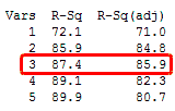
You might want to include only three predictors in this model. In my last blog, we saw how an under-specified model (one that was too simple) can produce biased estimates. However, an overspecified model (one that's too complex) is more likely to reduce the precision of coefficient estimates and predicted values. Consequently, you don’t want to include more terms in the model than necessary. (Read an example of using Minitab’s Best Subsets Regression.)
Finally, a different use for the adjusted R-squared is that it provides an unbiased estimate of the population R-squared.

What Is the Predicted R-squared?
The predicted R-squared indicates how well a regression model predicts responses for new observations. This statistic helps you determine when the model fits the original data but is less capable of providing valid predictions for new observations. (Read an example of using regression to make predictions.)
Minitab calculates predicted R-squared by systematically removing each observation from the data set, estimating the regression equation, and determining how well the model predicts the removed observation. Like adjusted R-squared, predicted R-squared can be negative and it is always lower than R-squared.
Even if you don’t plan to use the model for predictions, the predicted R-squared still provides crucial information.
A key benefit of predicted R-squared is that it can prevent you from overfitting a model. As mentioned earlier, an overfit model contains too many predictors and it starts to model the random noise.
Because it is impossible to predict random noise, the predicted R-squared must drop for an overfit model. If you see a predicted R-squared that is much lower than the regular R-squared, you almost certainly have too many terms in the model.
Examples of Overfit Models and Predicted R-squared
You can try these examples for yourself using this Minitab project file that contains two worksheets. If you want to play along and you don't already have it, please download the free 30-day trial of Minitab Statistical Software!
There’s an easy way for you to see an overfit model in action. If you analyze a linear regression model that has one predictor for each degree of freedom, you’ll always get an R-squared of 100%!
In the random data worksheet, I created 10 rows of random data for a response variable and nine predictors. Because there are nine predictors and nine degrees of freedom, we get an R-squared of 100%.
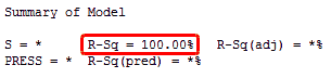
It appears that the model accounts for all of the variation. However, we know that the random predictors do not have any relationship to the random response! We are just fitting the random variability.
That’s an extreme case, but let’s look at some real data in the President's ranking worksheet.
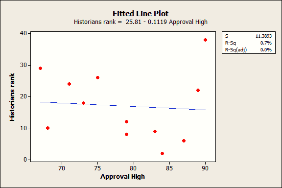
These data come from my post about great Presidents. I found no association between each President’s highest approval rating and the historian’s ranking. In fact, I described that fitted line plot (below) as an exemplar of no relationship, a flat line with an R-squared of 0.7%!
Let’s say we didn’t know better and we overfit the model by including the highest approval rating as a cubic polynomial.
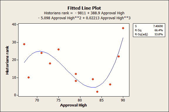
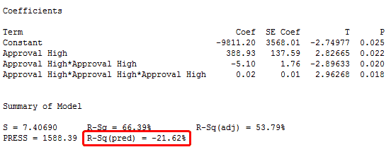
Wow, both the R-squared and adjusted R-squared look pretty good! Also, the coefficient estimates are all significant because their p-values are less than 0.05. The residual plots (not shown) look good too. Great!
Not so fast...all that we're doing is excessively bending the fitted line to artificially connect the dots rather than finding a true relationship between the variables.
Our model is too complicated and the predicted R-squared gives this away. We actually have a negative predicted R-squared value. That may not seem intuitive, but if 0% is terrible, a negative percentage is even worse!
The predicted R-squared doesn’t have to be negative to indicate an overfit model. If you see the predicted R-squared start to fall as you add predictors, even if they’re significant, you should begin to worry about overfitting the model.
Closing Thoughts about Adjusted R-squared and Predicted R-squared
All data contain a natural amount of variability that is unexplainable. Unfortunately, R-squared doesn’t respect this natural ceiling. Chasing a high R-squared value can push us to include too many predictors in an attempt to explain the unexplainable.
In these cases, you can achieve a higher R-squared value, but at the cost of misleading results, reduced precision, and a lessened ability to make predictions.
Both adjusted R-squared and predicted R-square provide information that helps you assess the number of predictors in your model:
- Use the adjusted R-square to compare models with different numbers of predictors
- Use the predicted R-square to determine how well the model predicts new observations and whether the model is too complicated
Regression analysis is powerful, but you don’t want to be seduced by that power and use it unwisely!
If you're learning about regression, read my regression tutorial!