


In statistics, t-tests are a type of hypothesis test that allows you to compare means. They are called t-tests because each t-test boils your sample data down to one number, the t-value. If you understand how t-tests calculate t-values, you’re well on your way to understanding how these tests work.
In this series of posts, I'm focusing on concepts rather than equations to show how t-tests work. However, this post includes two simple equations that I’ll work through using the analogy of a signal-to-noise ratio.
Minitab Statistical Software offers the 1-sample t-test, paired t-test, and the 2-sample t-test. Let's look at how each of these t-tests reduce your sample data down to the t-value.
How 1-Sample t-Tests Calculate t-Values
Understanding this process is crucial to understanding how t-tests work. I'll show you the formula first, and then I’ll explain how it works.
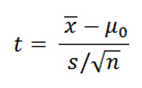
Please notice that the formula is a ratio. A common analogy is that the t-value is the signal-to-noise ratio.
Signal (a.k.a. the effect size)
The numerator is the signal. You simply take the sample mean and subtract the null hypothesis value. If your sample mean is 10 and the null hypothesis is 6, the difference, or signal, is 4.
If there is no difference between the sample mean and null value, the signal in the numerator, as well as the value of the entire ratio, equals zero. For instance, if your sample mean is 6 and the null value is 6, the difference is zero.
As the difference between the sample mean and the null hypothesis mean increases in either the positive or negative direction, the strength of the signal increases.

Lots of noise can overwhelm the signal.
Noise
The denominator is the noise. The equation in the denominator is a measure of variability known as the standard error of the mean. This statistic indicates how accurately your sample estimates the mean of the population. A larger number indicates that your sample estimate is less precise because it has more random error.
This random error is the “noise.” When there is more noise, you expect to see larger differences between the sample mean and the null hypothesis value even when the null hypothesis is true. We include the noise factor in the denominator because we must determine whether the signal is large enough to stand out from it.
Signal-to-Noise ratio
Both the signal and noise values are in the units of your data. If your signal is 6 and the noise is 2, your t-value is 3. This t-value indicates that the difference is 3 times the size of the standard error. However, if there is a difference of the same size but your data have more variability (6), your t-value is only 1. The signal is at the same scale as the noise.
In this manner, t-values allow you to see how distinguishable your signal is from the noise. Relatively large signals and low levels of noise produce larger t-values. If the signal does not stand out from the noise, it’s likely that the observed difference between the sample estimate and the null hypothesis value is due to random error in the sample rather than a true difference at the population level.
A Paired t-test Is Just A 1-Sample t-Test
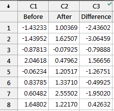
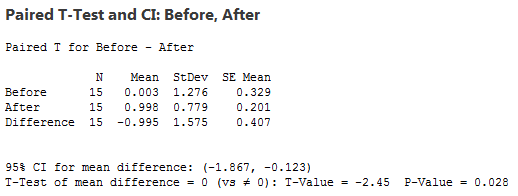
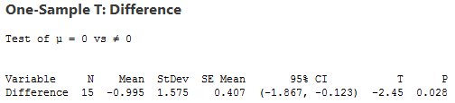
Many people are confused about when to use a paired t-test and how it works. I’ll let you in on a little secret. The paired t-test and the 1-sample t-test are actually the same test in disguise! As we saw above, a 1-sample t-test compares one sample mean to a null hypothesis value. A paired t-test simply calculates the difference between paired observations (e.g., before and after) and then performs a 1-sample t-test on the differences.
You can test this with this data set to see how all of the results are identical, including the mean difference, t-value, p-value, and confidence interval of the difference.
Understanding that the paired t-test simply performs a 1-sample t-test on the paired differences can really help you understand how the paired t-test works and when to use it. You just need to figure out whether it makes sense to calculate the difference between each pair of observations.
For example, let’s assume that “before” and “after” represent test scores, and there was an intervention in between them. If the before and after scores in each row of the example worksheet represent the same subject, it makes sense to calculate the difference between the scores in this fashion—the paired t-test is appropriate. However, if the scores in each row are for different subjects, it doesn’t make sense to calculate the difference. In this case, you’d need to use another test, such as the 2-sample t-test, which I discuss below.
Using the paired t-test simply saves you the step of having to calculate the differences before performing the t-test. You just need to be sure that the paired differences make sense!
When it is appropriate to use a paired t-test, it can be more powerful than a 2-sample t-test. For more information, go to Overview for paired t.
How Two-Sample T-tests Calculate T-Values
The 2-sample t-test takes your sample data from two groups and boils it down to the t-value. The process is very similar to the 1-sample t-test, and you can still use the analogy of the signal-to-noise ratio. Unlike the paired t-test, the 2-sample t-test requires independent groups for each sample.
The formula is below, and then some discussion.
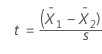
For the 2-sample t-test, the numerator is again the signal, which is the difference between the means of the two samples. For example, if the mean of group 1 is 10, and the mean of group 2 is 4, the difference is 6.
The default null hypothesis for a 2-sample t-test is that the two groups are equal. You can see in the equation that when the two groups are equal, the difference (and the entire ratio) also equals zero. As the difference between the two groups grows in either a positive or negative direction, the signal becomes stronger.
In a 2-sample t-test, the denominator is still the noise, but Minitab can use two different values. You can either assume that the variability in both groups is equal or not equal, and Minitab uses the corresponding estimate of the variability. Either way, the principle remains the same: you are comparing your signal to the noise to see how much the signal stands out.
Just like with the 1-sample t-test, for any given difference in the numerator, as you increase the noise value in the denominator, the t-value becomes smaller. To determine that the groups are different, you need a t-value that is large.
What Do t-Values Mean?
Each type of t-test uses a procedure to boil all of your sample data down to one value, the t-value. The calculations compare your sample mean(s) to the null hypothesis and incorporates both the sample size and the variability in the data. A t-value of 0 indicates that the sample results exactly equal the null hypothesis. In statistics, we call the difference between the sample estimate and the null hypothesis the effect size. As this difference increases, the absolute value of the t-value increases.
That’s all nice, but what does a t-value of, say, 2 really mean? From the discussion above, we know that a t-value of 2 indicates that the observed difference is twice the size of the variability in your data. However, we use t-tests to evaluate hypotheses rather than just figuring out the signal-to-noise ratio. We want to determine whether the effect size is statistically significant.
To see how we get from t-values to assessing hypotheses and determining statistical significance, read the other post in this series, Understanding t-Tests: t-values and t-distributions.