


If you read my blogs regularly, you’ll know that I’ve extensively used and written about linear models. We added a ton of features to Minitab that expand and enhance many types of linear models. I’m thrilled!
In this post, I want to share with my fellow analysts these linear model features and the benefits that they provide.
Linear Model Analyses in Minitab
Poisson Regression: If you have a response variable that is a count, you need Poisson Regression! For example, use Poisson Regression to model the count of failures or defects.
Stability Studies: Analyze the stability of a product over time and determine its shelf life. We’ve even included a worksheet generator to create a data collection plan! For example, use Stability Studies to model drug effectiveness by batch across time.
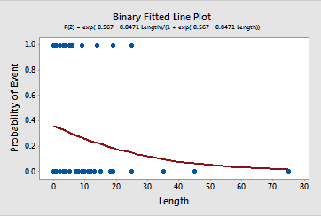 Binary Fitted Line Plot: This plot is similar to the existing fitted line plot, but for binary response variables. If you have a single predictor and need to graph the event probabilities for a binary response, this new graph effectively presents this information more clearly than ever!
Consistent Features across Linear Model Analyses
The interface and functionality have also been both improved and standardized across many types of models. Previously, some features were only available for a specific type of linear model. For example, you could only perform stepwise regression in Regression, and you could only use the Response Optimizer in DOE.
We made significant improvements to the following types of linear models:
- Factorial Designs
- General Full Factorial Designs
- Analyze Variability
- Response Surface Designs
- General Linear Models (GLM)
- Regression
- Binary Logistic Regression
- Poisson Regression
Thanks to the standardization across model types, all of the features I describe below apply to all of the above analyses! Pretty cool!
Easier to Specify Your Model
If your linear model has a lot of interactions and higher-order terms, you’ll love our new and improved interface for specifying the terms you need in your model. Additionally, you now have the ability to specify non-hierarchical models if you choose.
As an added convenience, we’ve also added the stepwise model selection procedure to all of the linear model analyses that I listed above. You also have greater control over how Minitab adds and removes terms from your model during this procedure.
Automatically Store Models for Later Use
It’s now a piece of cake to specify the best model for your data, but that’s often just the first step. If you need to use your model for additional tasks, you’ll come to love our stored models because they make it easy to perform important follow-up analyses!
In order to improve your workflow, we’ve introduced both the automatic ability to store models and a set of post-analyses to use with the stored models.
Every time you fit a model for one of analyses listed above, it gets stored right in the worksheet. After you settle on the perfect model, you can use the stored model to perform all of the post-analyses tasks below.
Post-Analyses that use Stored Linear Models
Prediction
There’s a cool interface that makes it much easier to enter the values that you want to predict!
Factorial Plots
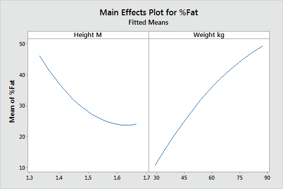 The main effects plot and interactions plot are available for types of linear models that they weren't before. Even cooler is the ability to produce these plots for continuous variables, rather than just categorical variables! This ability is particularly helpful when you want to understand interactions between continuous variables, which are to notoriously difficult to interpret using the numerical output.
This main effects plot is based on continuous variables. Notice how it reflects the curvature in the model!
Contour Plots and Surface Plots
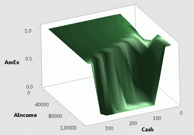 You can now generate both of these plots based on your stored model for all the model types listed above. The z-axis generally represents the fitted response value. However, what’s super cool is that for binary logistic regression, the z-axis represents the expected event probability!
In this surface plot based on a binary logistic model, we see how students’ finances affect their probability of carrying a credit card.
Overlaid Contour Plots
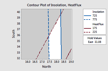 The overlaid contour plot based on multiple models is available for all of the listed model types. Overlaid contour plots display contour plots for multiple responses in a single graph.
Applications that involve multiple response variables present a different challenge than single response studies. Optimal variable values for one response may be far from optimal for another response. Overlaid contour plots allow you to visually identify an area of compromise among the various responses.
In this overlaid contour plot, the white region represents the combination of predictor values that yield satisfactory fitted values for both response variables.
Response Optimizer
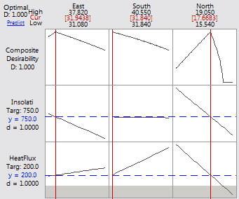 The Response Optimizer is now available for all of the listed model types. This tool is an even more advanced method to identify the combination of input variables that jointly optimize a set of response variables. Minitab calculates an optimal solution and produces the interactive optimization plot.
This plot allows you to interactively change the input variable settings to perform sensitivity analyses and possibly improve upon the initial solution. The session window output contains more detailed information about the optimal settings and the predicted outcomes.