For my last several posts, I’ve been writing about the problems associated with variability. First, I showed how variability is bad for customers. Next, I showed how variability is generally harder to control than the mean. In this post, I’ll show yet one more way that variability causes problems!
Variability can dramatically reduce your statistical power during hypothesis testing. Statistical power is the probability that a test will detect a difference (or effect) that actually exists.
It’s always a good practice to understand the variability present in your subject matter and how it impacts your ability to draw conclusions. Even when you can't reduce the variability, you can plan accordingly in order to assure that your study has adequate power.
(As a bonus for readers of this blog, this post contains the information necessary to solve the mystery that I will pose in my first post of the new year!)
How Variability Affects Statistical Power
Higher variability reduces your ability to detect statistical significance. But how?
The probability distribution plots below illustrate how this works. These three plots represent cases where we would use 2-sample t tests to determine whether the two populations have different means. These plots represent entire populations so we know that the 3 pairs of populations are truly different. However, for statistical analysis, we almost always use samples from the population, which provides a fuzzier picture.
For random samples, increasing the sample size is like increasing the resolution of a picture of the populations. With just a few samples, the picture is so fuzzy that we’d only be able to see differences between the most distinct of populations. However, if we collect a very large sample, the picture becomes sharp enough to determine the difference between even very similar populations.
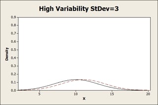
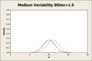
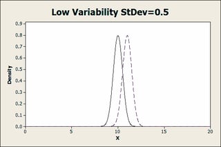
Each plot below displays two populations that we are studying. For all plots, the two populations have the same two means of 10 and 11, but different standard deviations, so the mean difference between all pairs of populations is always 1.
When the populations in these graphs are less visually distinct, we need higher resolution in our picture (i.e., a larger sample) to detect the difference.
For the high variability group, the 2 populations are virtually indistinguishable. It’s going to take a fairly high resolution to see this difference.
For the medium group, we can start to see the populations separating:
Finally, with low variability, there are two pretty distinct populations. We’d be able to see this difference even with a fairly low resolution.
Power and Sample Size
The graphs are visual representations but we can quantify how difficult it is to detect these differences with Minitab’s power and sample size calculations. To do this, we’ll look at the Power and Sample Size for 2-sample t. Normally, we’d enter estimates about the population because you almost never know the true population values (parameters in statistical parlance). However, we’re setting up these populations so we know the true values in this case.
So, for the high-variability population we’ll fill in the dialog box like this. To follow along in Minitab, go to: Stat > Power and Sample Size > 2-sample t.
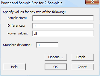
We leave the sample size field empty because we want Minitab to calculate this value. The difference and standard deviation fields are based on the populations that we set up. The power value is the likelihood that the test will detect the difference when one truly exists. 80% (0.8) is a fairly standard value but it varies by discipline, as we shall see. We get the following output:
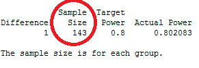
The Minitab output shows us that we’d need 143 samples for each of the two groups (286 total) to have an 80% chance of detecting the difference between the 2 high variability populations. That’s quite a few samples, which costs money! Let’s see what happens when we look at the populations that have less variability. Repeating what we did above, Minitab shows that you need:
- High variability: 286 total
- Medium variability: 74 total
- Low variability: 12 total
As you can see, the sample size that you need to have an 80% chance of detecting the same difference between the means drops dramatically with less variability.
Now, suppose you decided that you really wanted a 90% chance of detecting the difference, just to be extra certain? We’ll change the power value from 0.8 to 0.9 and compare the high to low variability populations. Minitab shows that you need:
- High: 286 increases to 382
- Low: 12 increases to 14
For the high variability scenario, you need nearly 100 additional samples to get that extra 10% of assurance, whereas you only need 2 more with low variability! This shows how it is much easier to obtain higher power values when you have lower variability.
Studies in physical sciences and engineering tend to involve very tight distributions. Therefore, these studies are often required to have a power value of 90%. However, the social sciences often deal with more variable properties (like personality assessments) that produce wider distributions. Consequently, social science studies often have a somewhat lower requirement for power, 70 or 80%.
Conclusion: Why It's All About Variability
Power and sample size estimates are only as good as your estimate of the variability (standard deviation). Unfortunately, estimating the variability is often the most difficult part. To obtain this estimate, you may have to rely on the literature, pilot studies, or even educated guesses. Even then, you might get it wrong. But as you conduct more studies in an area, your estimate of the variability should become more precise. It's a process.
I'm sure that it's obvious that you should always calculate power and sample size before a study to avoid conducting a low-power analysis, and Minitab makes this very easy to do. But you should also assess power after a study that produced insignificant results. This time, use the standard deviation estimate from the sample data, which may be more accurate than the pre-study estimate.
Imagine that we conducted a study, assumed the medium variability scenario, and used a sample size of 74. We'd think that our study had 80% power. Sadly, we get insignificant results. However, we notice that our actual sample variability is higher than our pre-study estimate. In fact, it is consistent with the high variability scenario. When we recompute power, it turns out that our power was only 52%! The low power might explain the insignificant results.
Fortunately, we can use this new estimate to produce an improved study! Then, with a sample size we know we can rely on, we can all sing along with I've Got the Power!


