


Multicollinearity is problem that you can run into when you’re fitting a regression model, or other linear model. It refers to predictors that are correlated with other predictors in the model. Unfortunately, the effects of multicollinearity can feel murky and intangible, which makes it unclear whether it’s important to fix.
My goal in this blog post is to bring the effects of multicollinearity to life with real data! Along the way, I’ll show you a simple tool that can remove multicollinearity in some cases.
How Problematic is Multicollinearity?
Moderate multicollinearity may not be problematic. However, severe multicollinearity is a problem because it can increase the variance of the coefficient estimates and make the estimates very sensitive to minor changes in the model. The result is that the coefficient estimates are unstable and difficult to interpret. Multicollinearity saps the statistical power of the analysis, can cause the coefficients to switch signs, and makes it more difficult to specify the correct model.
Do I Have to Fix Multicollinearity?
The symptoms sound serious, but the answer is both yes and no—depending on your goals. (Don’t worry, the example we'll go through next makes it more concrete.) In short, multicollinearity:
- can make choosing the correct predictors to include more difficult.
- interferes in determining the precise effect of each predictor, but...
- doesn’t affect the overall fit of the model or produce bad predictions.
Depending on your goals, multicollinearity isn’t always a problem. However, because of the difficulty in choosing the correct model when severe multicollinearity is present, it’s always worth exploring.
The Regression Scenario: Predicting Bone Density
I’ll use a subset of real data that I collected for an experiment to illustrate the detection, effects, and removal of multicollinearity. You can read about the actual experiment here. (If you're not already using it, please download the free trial of Minitab and play along!)
We’ll use Regression to assess how the predictors of physical activity, percent body fat, weight, and the interaction between body fat and weight are collectively associated with the bone density of the femoral neck.
Given the potential for correlation among the predictors, we’ll have Minitab display the variance inflation factors (VIF), which indicate the extent to which multicollinearity is present in a regression analysis. A VIF of 5 or greater indicates a reason to be concerned about multicollinearity.
General Regression Results
Here are the results of the Minitab analysis:
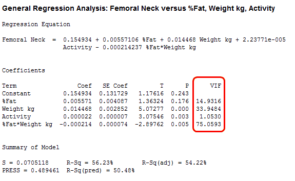
In the results above, Weight, Activity, and the interaction term are significant while %Fat is not significant. However, three of the VIFs are very high because they are well over 5. These values suggest that the coefficients are poorly estimated and we should be wary of their p-values.
Standardize the Continuous Predictors
In this model, the VIFs are high because of the interaction term. Interaction terms and higher-order terms (e.g., squared and cubed predictors) are correlated with main effect terms because they include the main effects terms.
To reduce high VIFs produced by interaction and higher-order terms, you can standardize the continuous predictor variables. In Minitab, it’s easy to standardize the continuous predictors by clicking the Coding button in Regression dialog box and choosing the standardization method.
For our purposes, we’ll choose the Subtract the mean method, which is also known as centering the variables. This method removes the multicollinearity produced by interaction and higher-order terms as effectively as the other standardization methods, but it has the added benefit of not changing the interpretation of the coefficients. If you subtract the mean, each coefficient continues to estimate the change in the mean response per unit increase in X when all other predictors are held constant.
I’ve already added the standardized predictors in the worksheet we’re using; they're in the columns that have an S added to the name of each standardized predictor.
Regression with Standardized Predictors
We’ll fit the same model as before, but this time using the standardized predictors.
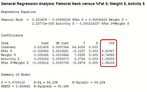
In the model with the standardized predictors, the VIFs are down to an acceptable range.
Comparing Regression Models to See the Effects of Multicollinearity
Because standardizing the predictors effectively removed the multicollinearity, we could run the same model twice, once with severe multicollinearity and once with moderate multicollinearity. This provides a great head-to-head comparison and it reveals the classic effects of multicollinearity.
The standard error of the coefficient (SE Coef) indicates the precision of the coefficient estimates. Smaller values represent more reliable estimates. In the second model, you can see that the SE Coef is smaller for both %Fat and Weight. Also, %Fat is significant this time, while it was insignificant in the model with severe multicollinearity. Also, its sign has switched from + 0.005 to – 0.005! The %Fat estimate in both models is about the same absolute distance from zero, but it is only significant in the second model because the estimate is more precise.
Compare the Summary of Model statistics between the two models and you’ll notice that S, R-squared, adjusted R-squared, and the others are all identical. Multicollinearity doesn’t affect how well the model fits. In fact, if you want to use the model to make predictions, both models produce identical results for fitted values and prediction intervals!
Multicollinear Thoughts
Multicollinearity can cause a number of problems. We saw how it sapped the significance of one of our predictors and changed its sign. Imagine trying to specify a model with many more potential predictors. If you saw signs that kept changing and incorrect p-values, it could be hard to specify the correct model! Stepwise regression does not work as well with multicollinearity.
However, we also saw that multicollinearity doesn’t affect how well the model fits. If the model satisfies the residual assumptions and has a satisfactory predicted R-squared, even a model with severe multicollinearity can produce great predictions.
You also don’t have to worry about every single pair of predictors that has a high correlation. When putting together the model for this post, I thought for sure that the high correlation between %Fat and Weight (0.827) would produce severe multicollinearity all by itself. However, that correlation only produced VIFs around 3.2. So don’t be afraid to try correlated predictors—just be sure to check those VIFs!
For our model, the severe multicollinearity was primarily caused by the interaction term. Consequently, we were able to remove the problem simply by standardizing the predictors. However, when standardizing your predictors doesn’t work, you can try other solutions such as:
- removing highly correlated predictors
- linearly combining predictors, such as adding them together
- running entirely different analyses, such as partial least squares regression or principal components analysis
When considering a solution, keep in mind that all remedies have potential drawbacks. If you can live with less precise coefficient estimates, or a model that has a high R-squared but few significant predictors, doing nothing can be the correct decision because it won't impact the fit.
If you're learning about regression, read my regression tutorial!