


Making parts that are truly interchangeable is a critical aspect of modern manufacturing. The same parts may be manufactured in different plants spread around the globe or by suppliers located far away. Parts need to be manufactured to specifications to ensure that they are almost identical to allow an easy assembly of new products.
Interchangeability is increasingly important in the service industry as well. Because customers expect similar standards from a service company wherever it does business around the globe, best practices need to be deployed throughout a company and different subsidiaries need to interact on a common basis.
The objective of this post is to show how you can set a tolerance interval on an input (a parameter of a part) when you need an output (a parameter of the final assembled product) to remain well within specifications. You can achieve this using a very simple tool: the prediction intervals of a regression model.
A Historical Perspective on Interchangeable Parts
Historically, the firearms industry has played an important role in making the concept of standardized specifications an established practice.
In the late 18th century, the French gunsmith Honoré LeBlanc advocated the use of standardized designs and interchangeable parts so that guns could be easily repaired if broken. Gun parts were still carefully made by highly skilled craftsmen, though.
Making guns with truly standardized parts was very hard to achieve, but the military really wanted to be able to interchange gun parts. Why? When a gun failed in the battlefield, a soldier could quickly replace a damaged part and keep on fighting. Also, many handmade guns had unreliable performance records.
Eli Whitney demonstrated this interchangeability concept right in front of the United States Congress. He brought 10 guns to the capitol, disassembled them into their single components, mixed the parts, and then reassembled the guns back together.
By the late 19th century, engineers with armory experience had spread interchangeable manufacturing techniques to other American industries.
Determining Tolerance Windows
Setting tolerances that are not too wide and not too tight is critical. Tolerances that are too wide may generate unstable behaviors in the final product, and hence quality problems. Tolerances that are too tight are difficult to deal with at a manufacturing level, and hence increase final costs.
Assembly specifications often reflect the Voice Of the Customer (VOC), but how can we convert these assembly specifications into tolerances for individual components ?
Consider the graph below. A paint manufacturer conducted an experiment to better understand the relationship between stir rate and impurity level. Increasing the stir rate can cause the pigment in paint to coagulate. These impurities negatively affect the paint performance. This is a fitted line plot (from a regression analysis) that shows the effect of Stir Rate on impurity.
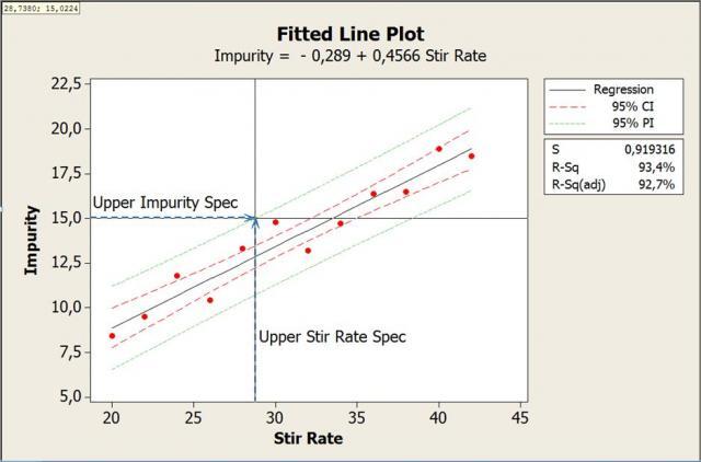
The fitted line plot illustrates the way in which a faster Stir Rate actually increases the amount of impurities in the paint. According to the regression equation, an increase of 1 unit in the Stir Rate generates an increase of 0.4566 in the impurity level.
Now let us go one step further: If we need to ensure that the level of impurity is not larger than 15, how can we set tolerances on the Stir Rate variable ?
In the diagram above, the Prediction Interval (the area between the green lines) graphically represents the natural spread of individual values around the regression line. To account for this uncontrollable variability (caused by process and measurement variations as well environmental fluctuations, etc.) we need to consider the upper bound of the Prediction Interval (PI).
When the upper bound value is equal to 15 (on the Y scale), it corresponds to a Stir Rate value of 28.73 (on the X scale). In Minitab, the Crosshairs functionality can be used to identify the input value that actually corresponds to an output value of 15 on the upper prediction interval bound. Right-click on the graph and choose Crosshairs in the list, then move the cross to the exact point where the upper bound of the prediction interval crosses the 15 value on the impurity scale.
The 28.73 value can be considered as an upper specification limit of the Stir Rate so that the amount of impurity is kept well under 15. In the graph a 95% Prediction interval (PI) has been used. This is the default value in Minitab, but it can be modified to a 99% prediction interval to better protect the customer.
Displaying the Prediction Interval
In this context, we are only interested in the prediction interval (PI), which reflects the variability in the individual values, not in the confidence interval (CI) which represents the precision of the regression model parameter estimates.
In Minitab, to display the Prediction interval (PI) in a graph go to Stat > Regression > Fitted line Plot. In the Fitted Line Plot dialogue box, click on Option and check the Display Prediction Interval box. The confidence level may also be modified from the default value of 95%.
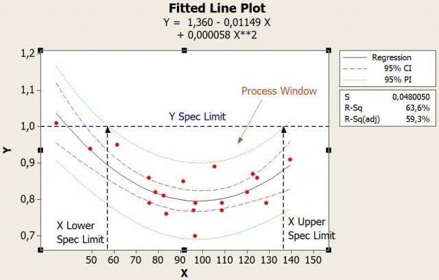
In the graph below, we clearly have a quadratic effect of the input, and so a quadratic regression model has been used. We would like the output (the Y) not to exceed a certain value. This time, lower and an upper specification limits on the input (the X) need to be set so that the resulting output is kept below its specification value.
Again the upper bound of the prediction interval is used to account for the variations in the individual values, in order to define a process window.
Conclusion
This approach is very similar to Shainin’s Isoplot technique. It is very simple and intuitive, and can be used whenever you need to specify a process window for a single component that affects the final output.
Often, however, the output will be affected by changes in several components of an assembled product, in this case, more advanced techniques are required, such as designed experiments (DOE) and Monte Carlo techniques.