In honor of the 100^th anniversary of the sinking of the Titanic, we recently posted a dataset on the passengers aboard the ship that included Class (coach or first), Gender (female or male), Age, and Status (survived or died).  From Age an additional column was created indicating Child (17 years or younger) or Adult (18 years or older).

In an earlier post, we showed how survival rates could be compared between levels of one variable—for example, females versus males—using Stat > Tables > Cross Tabulation and Chi Square.  But what if we wanted to take all factors into consideration to paint a complete picture of survival rates?

Applying Binary Logistic Regression

In Minitab Statistical Software, Stat > Regression > Binary Logistic Regression allows us to create models when the response of interest (Status, in this case) is binary and only takes two values. To begin, include all terms and two-way interactions in the model and reduce it from there:

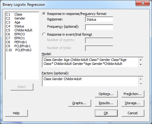
By clicking on Options, choose whether the model will predict the odds of Status = “Died” or Status = “Survived”…as an optimist, I chose “Survived”:

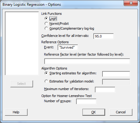
You can also try different Link Functions in Options to find the model that best fits your data.  By removing terms from my model that are not statistically significant and choosing different Link Functions, I ultimately came up with this Logistic Regression Table, similar to an ANOVA table from typical ANOVA (Stat > ANOVA) or Regression (Stat > Regression) output in Minitab:

Logistic Regression Table

Predictor           Coef    SE Coef      Z      P
Constant       -0.191839   0.175568   -1.09   0.275
Class
First           0.971320  0.0952002   10.20   0.000
Gender
Male            -1.03799   0.200630   -5.17   0.000
Age            0.0044963  0.0033885    1.33   0.185
ChildorAdult
Child           0.387517   0.174976    2.21   0.027
Gender*Age
Male          -0.0123825  0.0040596   -3.05   0.002

Goodness-of-Fit Tests

Method           Chi-Square   DF      P
Pearson             270.946  272  0.507
Deviance            313.073  272  0.044
Hosmer-Lemeshow       8.815    8  0.358

For these tests, a significant p-value indicates our model does not fit the data adequately.  While we do have one significant test (Deviance), the other two tests provide no evidence of significance and we are fairly comfortable that our model provides a good fit.  If you find you have significant terms but the Goodness-of-Fit Tests are showing an inadequate model fit, it may be worth trying a different Link Function back in the Option dialog.  In this case, I found the Gompit link function to provide the best fit.

Measures of Association to Assess the Regression Model

Finally, we can assess our model using Measures of Association:

Measures of Association:
(Between the Response Variable and Predicted Probabilities)

Pairs        Number  Percent  Summary Measures
Concordant   785712     74.2  Somers' D              0.49
Discordant   262124     24.7  Goodman-Kruskal Gamma  0.50
Ties          11554      1.1  Kendall's Tau-a        0.22
Total       1059390    100.0

Measures of Association compares how often passengers who survived had higher predicted odds of survival than passengers who did not survive.  By comparing every surviving passenger with every passenger who died, Minitab determines how often the model correctly or incorrectly predicted which would survive. In our analysis, 74.2% of the time the surviving passenger had higher predicted odds of survival, while 24.7% of the time they had lower and 1.1% of the time the odds were the same.  With a good model you want a high percentage of concordant pairs and a low percentage of discordant pairs.

Using the Regression Model to Predict Survival

Finally, back in the main Binary Logistic Regression dialog box,  choose Prediction and choose to store the predicted odds of survival for each passenger (shown below) or for new data points, as well as confidence intervals:

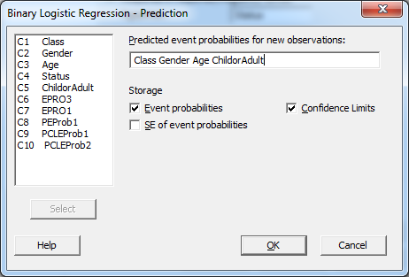
Using this information, I created a graph demonstrating the odds of survival for passengers aboard the Titanic based on all of our significant factors:

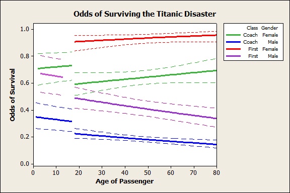
Interestingly, there was only one female child in the first-class cabin on that voyage, therefore we could not model the survival odds for female children in first-class.

Otherwise, it is clear from the graph that if you were an adult female in first class, your odds of survival were quite high and increased slightly if you were older. Even for an 18-year old female in first class, the odds of survival are estimated at 90.6% as compared to 32.3% for passengers in general!

Unlike females whose odds of survival increased with age, a male’s odds of survival decreased with age.  (Remember that Gender*Age interaction?)  So for an 80-year-old male passenger in coach, your odds of survival were a mere 14.4%!  See in the dataset that of the 25 passengers meeting this criteria, a mere 3 survived for a true rate of 12%, which is consistent with the model.

Had you been a male passenger who knew ahead of time about the impending tragedy, the cost of a first class ticket would have felt like a bargain. The same 80-year-old male would have enjoyed a relatively good 33.7% chance of survival had he booked in first class.

Likewise, taking this voyage as a 17-year-old who would have been boarded on a lifeboat instead of an 18-year-old who would remain on the sinking ship increases your odds of survival by 10-14%, depending on Gender and Class.

By looking at multiple factors at once, we are able to get a clear and accurate look at the odds of survival for any passenger based on just a few factors!