


In Part 1 of this blog series, I wrote about how statistical inference uses data from a sample of individuals to reach conclusions about the whole population. That’s a very powerful tool, but you must check your assumptions when you make statistical inferences. Violating any of these assumptions can result in false positives or false negatives, thus invalidating your results.
The common data assumptions are: random samples, independence, normality, equal variance, stability, and that your measurement system is accurate and precise.
I addressed random samples and statistical independence last time. Now let’s consider the assumptions of Normality and Equal Variance.
What Is the Assumption of Normality?
Before you perform a statistical test, you should find out the distribution of your data. If you don’t, you risk selecting an inappropriate statistical test. Many statistical methods start with the assumption your data follow the normal distribution, including the 1- and 2-Sample t tests, Process Capability, I-MR, and ANOVA. If you don’t have normally distributed data, you might use an equivalent non-parametric test based on the median instead of the mean, or try the Box-Cox or Johnson Transformation to transform your non-normal data into a normal distribution.
But keep in mind that many statistical tools based on the assumption of normality do not actually require normally distributed data if the sample sizes are at least 15 or 20. But if sample sizes are less than 15 and the data are not normally distributed, the p-value may be inaccurate and you should interpret the results with caution.
There are several methods to determine normality in Minitab, and I’ll discuss two of the tools in this post: the Normality Test and the Graphical Summary.
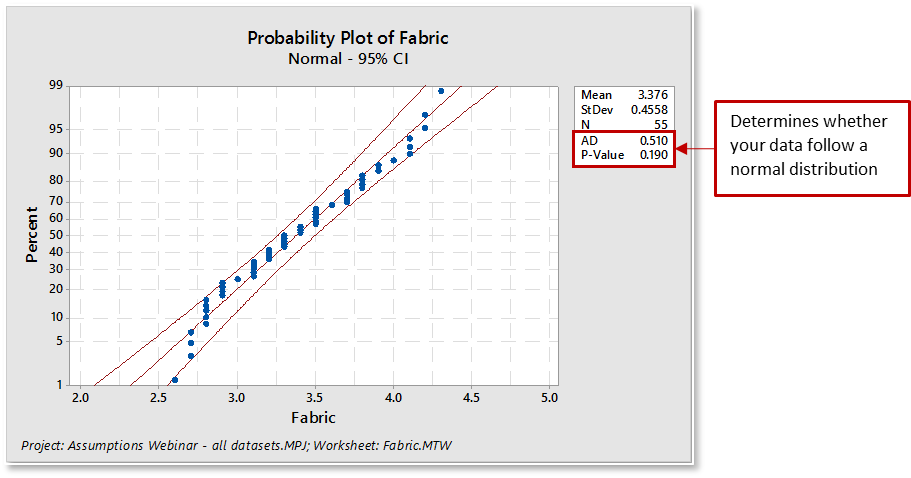
Minitab’s Normality Test will generate a probability plot and perform a one-sample hypothesis test to determine whether the population from which you draw your sample is non-normal. The null hypothesis states that the population is normal. The alternative hypothesis states that the population is non-normal.
Choose Stat > Basic Statistics > Normality Test
When evaluating the distribution fit for the normality test:
- The plotted points will roughly form a straight line. Some departure from the straight line at the tails may be okay as long as it stays within the confidence limits.
- The plotted points should fall close to the fitted distribution line and pass the “fat pencil” test. Imagine a "fat pencil" lying on top of the fitted line: If it covers all the data points on the plot, the data are probably normal.
- The associated Anderson-Darling statistic will be small.
- The associated p-value will be larger than your chosen α-level (commonly chosen levels for α include 0.05 and 0.10).
The Anderson-Darling statistic is a measure of how far the plot points fall from the fitted line in a probability plot. The statistic is a weighted squared distance from the plot points to the fitted line with larger weights in the tails of the distribution. For a specified data set and distribution, the better the distribution fits the data, the smaller this statistic will be.
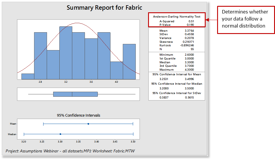
Minitab’s Descriptive Statistics with the Graphical Summary will generate a nice visual display of your data and calculate the Anderson-Darling & p-value. The graphical summary displays four graphs: histogram of data with an overlaid normal curve, boxplot, and 95% confidence intervals for both the mean and the median.
Choose Stat > Basic Statistics > Graphical Summary
 When interpreting a graphical summary report for normality:
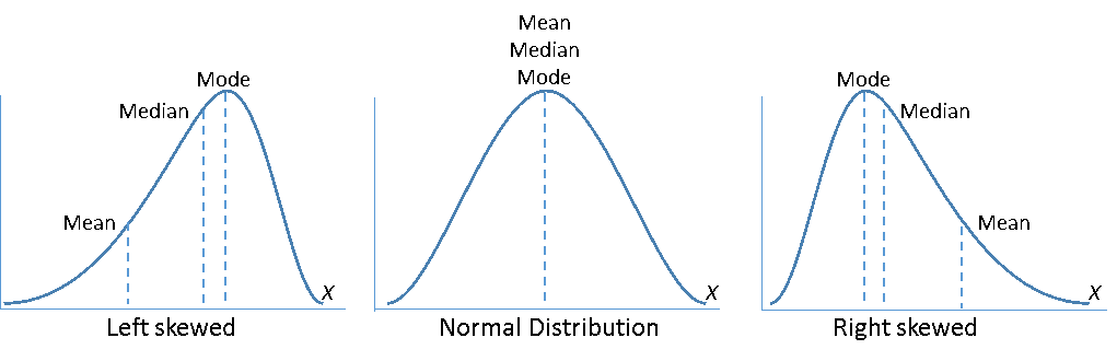
- The data will be displayed as a histogram. Look for how your data is distributed (normal or skewed), how the data is spread across the graph, and if there are outliers.
- The associated Anderson-Darling statistic will be small.
- The associated p-value will be larger than your chosen α-level (commonly chosen levels for α include 0.05 and 0.10).
For some processes, such as time and cycle data, the data will never be normally distributed. Non-normal data are fine for some statistical methods, but make sure your data satisfy the requirements for your particular analysis.
What Is the Assumption of Equal Variance?
In simple terms, variance refers to the data spread or scatter. Statistical tests, such as analysis of variance (ANOVA), assume that although different samples can come from populations with different means, they have the same variance. Equal variances (homoscedasticity) is when the variances are approximately the same across the samples. Unequal variances (heteroscedasticity) can affect the Type I error rate and lead to false positives. If you are comparing two or more sample means, as in the 2-Sample t-test and ANOVA, a significantly different variance could overshadow the differences between means and lead to incorrect conclusions.
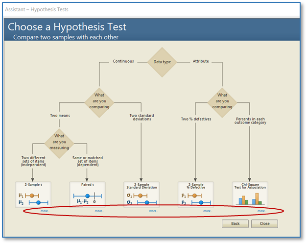
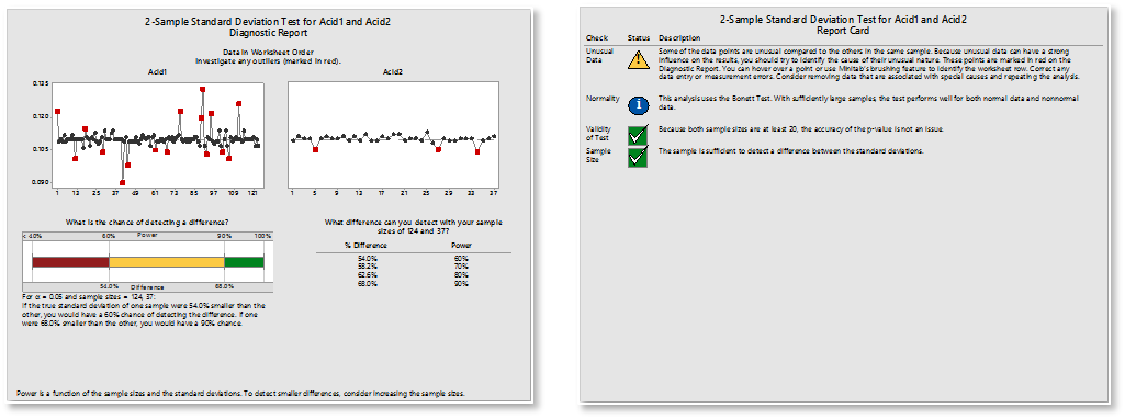
Minitab offers several methods to test for equal variances. Consult Minitab Help to decide which method to use based on the type of data you have. You can also use the Minitab Assistant to check this assumption for you. (Tip: When using the Assistant, click “more” to see data collection tips and important information about how Minitab calculates your results.)
After the analysis is performed, check the Diagnostic Report for the test interpretation and the Report Card for alerts to unusual data points or assumptions that were not met. (Tip: When performing the 2-Sample t test and ANOVA, the Assistant takes a more conservative approach and uses calculations that do not depend on the assumption of equal variance.)
The Real Reason You Need to Check the Assumptions
You will be putting a lot of time and effort into collecting and analyzing data. After all the work you put into the analysis, you want to be able to reach correct conclusions. Some analyses are robust to departures from these assumptions, but take the safe route and check! You want to be confident that you can tell whether observed differences between data samples are simply due to chance, or if the populations are indeed different!
It’s easy to put the cart before the horse and just plunge in to the data collection and analysis, but it’s much wiser to take the time to understand which data assumptions apply to the statistical tests you will be using, and plan accordingly.
In my next blog post, I will review the common assumptions about stability and the measurement system.