


See if this sounds fair to you. I flip a coin.
Heads: You win $1.
Tails: You pay me $1.
You may not like games of chance, but you have to admit it seems like a fair game. At least, assuming the coin is a normal, balanced coin, and assuming I’m not a sleight-of-hand magician who can control the coin.
How about this next game?
You pay me $2 to play.
I flip a coin over and over until it comes up heads.
Your winnings are the total number of flips.
So if the first flip comes up heads, you only get back $1. That’s a net loss of $1. If it comes up tails on the first flip and heads on the second flip, you get back $2, and we’re even. If it comes up tails on the first two flips and then heads on the third flip, you get $3, for a net profit of $1. If it takes more flips than that, your profit is greater.
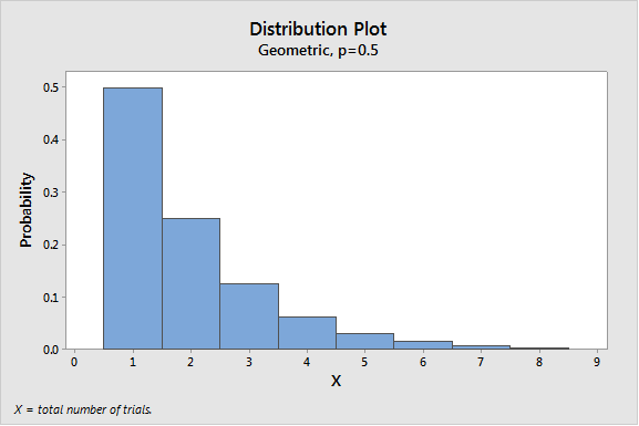
It’s not quite as obvious in this case, but this would be considered a fair game if each coin flip has an equal chance of heads or tails. That’s because the expected value (or mean) number of flips is 2. The total number of flips follows a geometric distribution with parameter p = ½, and the expected value is 1/p.
Now it gets really interesting. What about this next game?
You pay me $x dollars to play.
I flip a coin over and over until it comes up heads.
Your winnings start at $1, but double with every flip.
This is a lot like the previous game with two important differences. First, I haven’t told you how much you have to pay to play. I just called it x dollars. Second, the winnings grow faster with the number of flips. It starts off the same with $1 for one flip and $2 dollars for two flips. But then it goes to $4, then $8, then $16. If the first head comes up on the eighth flip, you win $128. And it just keeps getting better from there.
So what’s a fair price to play this game? Well, let’s consider the expected value of the winnings. It’s $∞. You read that right. It’s infinity dollars! So you shouldn’t be too worried about what x is, right? No matter what price I set, you should be eager to pay it. Right? Right?
I’m going to go out on a limb and guess that maybe you would not just let me name my price. Sure, you’d admit that it’s worth more than $2. But would you pay $10? $50? $100,000,000? If the fair price is the expected winnings, then any of these prices should be reasonable. But I’m guessing you would draw the line somewhere short of $100, and maybe even less than $10.
This fascinating little conundrum is known as the Saint Petersburg paradox. Wikipedia tells me it goes by that name because it was addressed in the Commentaries of the Imperial Academy of Science of Saint Petersburg back in 1738 by that pioneer of probability theory, Daniel Bernoulli.
The paradox is that while theory tells us that no price is too high to pay to play this game, nobody is willing to pay very much at all to play it.
What’s more, even if you decide what you're willing to pay, you won't find any casinos that even offer this game, because the ultimate outcome is just as unpredictable for the house as it is for the player.
The paradox has been discussed from various angles over the years. One reason I find it so interesting is that it forces me to think carefully about things that are easy to take for granted about the mean of a distribution.
Such as…
The mean is a measure of central tendency.
This is one of the first things we learn in statistics. The mean is in some sense a central value, which the data tends to vary around. It’s the balancing point of the distribution. But when the mean is infinite, this interpretation goes out the window. Now every possible value in the distribution is less than the mean. That’s not very central!
The sample mean approaches the population mean.
One of the most powerful results in statistics is the law of large numbers. Roughly speaking, it tells us that as your sample size grows, you can expect the sample average to approach the mean of the distribution you are sampling from. I think this is a good reason to treat the mean winnings as the fair price for playing the game. If you play repeatedly at the fair price your average profit approaches zero. But here’s the catch: the law of large numbers assumes the mean of the distribution is finite. So we lose one of the key justifications of treating the mean as the fair price when it’s infinite.
The central limit theorem.
Another extremely important result in statistics is the central limit theorem, which I wrote about in a previous blog post. It tells us that the average of a large sample has an approximate normal distribution centered at the population mean, with a standard deviation that shrinks as the sample size grows. But the central limit theorem requires not only a finite mean but a finite standard deviation. I’m sorry to tell you that if the mean of the distribution is infinite, then so is the standard deviation. So not only do we lack a finite mean that our average winnings can gravitate toward, we don’t have a nicely behaved standard deviation to narrow down the variability of our winnings.
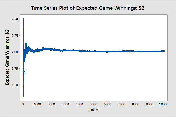
Let’s end by using Minitab to simulate these two games where the payoff is tied to the number of flips until heads comes up. I generated 10,000 random values from the geometric distribution. The two graphs show the running average of the winnings in the two games. In the first case, we have expected winnings of 2, and we see the average stabilizes near 2 pretty quickly.
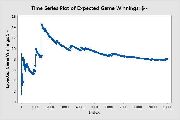
In the second case, we have infinite expected winnings, and the average does not stabilize.
If you'd like to do some simulation on this paradox yourself, here's how to do it in Minitab. First, use Calc > Make Patterned Data > Simple Set of Numbers... to make a column with the numbers 1 to 10,000. Next, open Calc > Random Data > Geometric... to create a separate column of 10,000 random data points from the geometric distribution, using .5 as the Event Probability.
Now we can compute the running average of the random geometric data in C2 with Minitab's Calculator, using the PARS function. PARS is short for “partial sum.” In each row it stores the sum of the data up to and including that row. To get the running average of a game where the expected winnings are $2, divide the partial sums by C1, which just contains the row numbers:
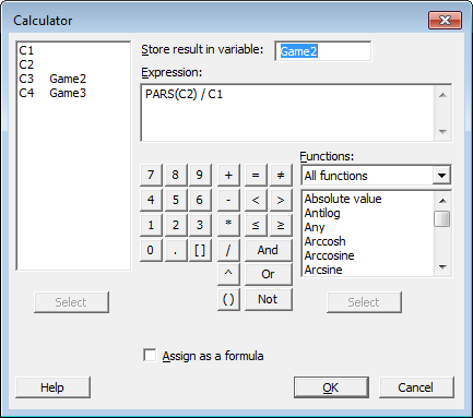
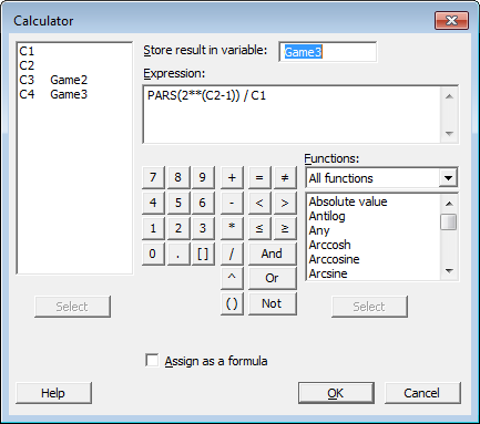
The computation for the game with infinite mean is the same, except that the winnings double in value when C2 increases by 1. Therefore, we take the partial sums of 2(C2 – 1) instead of just C2, and divide each by C1. That formula is entered in the calculator as shown below:
Finally, select Time Series Analysis > Time Series Plot... and plot the running average of the games with expected winnings of $2 and $∞.
So, how much would you pay to play this game?