


My previous post showed an example of using ordinary linear regression to model a count response. For that particular count data, shown by the blue circles on the dot plot below, the model assumptions for linear regression were adequately satisfied.
But frequently, count data may contain many values equal or close to 0. Also, the distribution of the counts may be right-skewed. In the quality field, this commonly occurs when you count the number of defects on each item, or the number of defectives in a sample.
So let's suppose that the number of ants coming to each sandwich portion was instead the count data shown by the red square symbols on the dot plot.

If you want to follow along, open the Minitab project file with the new count data. Set up and analyze the ordinary linear regression model the same way as in Part 1. You should get the following result:
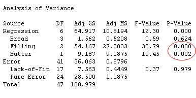
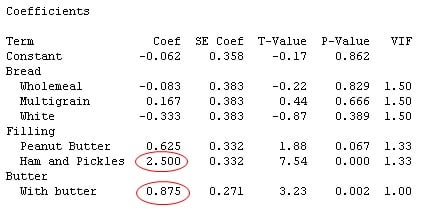
For the new count data, notice that the general relationship between the predictors and the count response are similar to those in the original data set. Both Filling and Butter are statistically significant predictors for the ant count response (p < 0.1). Similarly, as before, the coefficients table shows that Ham and Pickles, With Butter are the predictor levels associated with the highest ant count.
But for the new count data, look what happens to the regression equation:
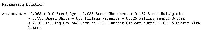
The equation now yields negative counts for some predictor values. For example, the estimated ant count for a Vegemite sandwich on white bread without butter is approximately -0.4. So if you drop that particular sandwich on a sidewalk in Australia, you can expect a little less than negative one-half of an ant to appear. A model that predicts antimatter. Hmm. Intriguing. But not very practical.
What about the model assumptions?
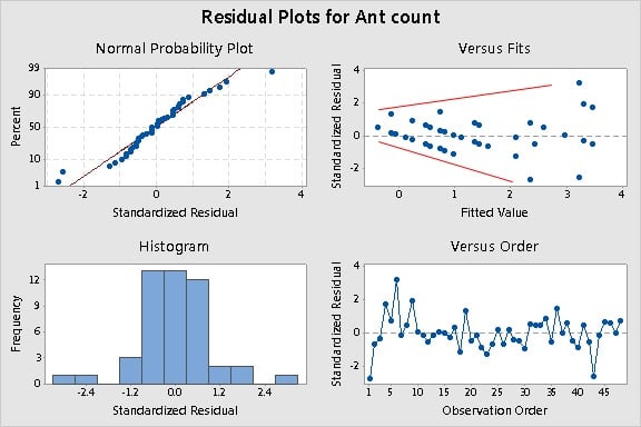
With the new count response data, the Residuals Versus Fits plot suggests that the critical assumption of constant variance may be violated. The spread of the residuals appears to increase as the fitted values of the model increase. This classic "megaphone" pattern in the residual plot is a problem—the model estimates get more erratic at higher fitted values.
When this happens, one common approach is to transform the response data to stabilize the variance. In fact, Minitab's linear regression analysis includes an option to perform a Box-Cox transformation (which is a family of power transformations that includes log transform, square root, and other transformation functions) for situations like this. But here's the catch: In many cases, count data can be problematic to transform, especially if they contain the value 0.
For example, try to perform the Box-Cox transformation in Minitab with the new count data, and you'll get this error message.
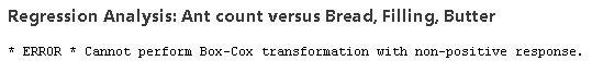
Even if you try a transformation that can handle counts of 0, you might run into problems due to poor discrimination in your count data. So, when you use ordinary linear regression with a count response, and one of the critical assumptions aren't met—you may find yourself up a creek without a log (or other) transform.
And even if your count data don't include 0, or you manage to find a transformation that works (or use sleight-of-hand to replace 0s in your data set with very minuscule decimal values to make all the data positive), the resulting model with the transformed values may still yield problematic estimates for a count response.
Now what?
Well, instead of using Alka Seltzer to clean your toilet bowl, how about using a product that'd been specifically designed to clean it, such as a toilet bowl cleaner?
That is, instead of using ordinary linear regression, which is technically designed to evaluate a continuous response, why not use a regression analysis specifically designed to analyze a count response? Stay tuned for the next post (Part 3).