


If you use ordinary linear regression with a response of count data, if may work out fine (Part 1), or you may run into some problems (Part 2).
Given that a count response could be problematic, why not use a regression procedure developed to handle a response of counts?
A Poisson regression analysis is designed to analyze a regression model with a count response.
First, let's try using Poisson regression on the count response composed mostly of small data values, including 0, which was so problematic to evaluate using ordinary linear regression. In Minitab, choose Stat > Regression > Poisson Regression > Fit Poisson Model and set up the regression model with the same three categorical predictors as before. The output includes the table shown below:
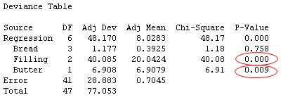
Filling and Butter are statistically significant at the 0.1 level—just as they were when using ordinary linear regression. But take a look at the regression equation:
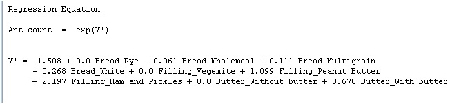
The regression equation is different for a Poisson model than for ordinary linear regression. For one thing, the estimated ant count response equals the exponentiated value of the Y' value given by the equation. For example, for a peanut butter sandwich on whole meal bread, with butter, the equation yields a Y' value of -1.508 - 0.061(1) + 1.099(1) + 0.670(1) = 0.2. But that's not the estimated ant count. The estimated ant count is exp (0.2) = e0.2 ≈ 1.22. (By the way, you can have Minitab perform this ugly number crunching for you: Choose Poisson Regression > Predict and fill in the predictor values for which you want a response estimate.)
Notice that with Poisson regression, the regression equation never produces a negative count response, as it can for ordinary linear regression. That's because even if the equation contains negative coefficients that produce a negative value of Y' for some values of the predictors, the exponentiated value of that negative value will always be positive. The smallest response estimate you can possibly get is essentially 0. That's a definite advantage of using Poisson regression with a count response—you don't have to grapple with those weird "antimatter" response estimates.
As with any regression analysis, Poisson regression has model assumptions that need to be evaluated, by examining the residual plots.
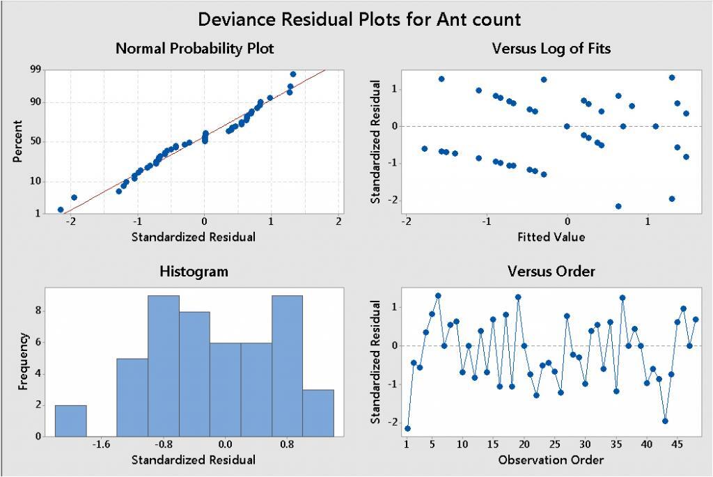
Here, the residual plots seem to be OK. The Residuals Versus Log of Fits plot shows a slight increasing pattern—but nothing as troublesome as the classic megaphone pattern we saw when we evaluated these data using ordinary linear regression in Part 2.
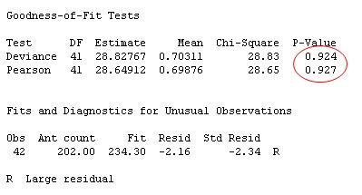
For Poisson regression, you should also examine the goodness-of-fit results in the Session window:
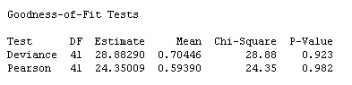
For the goodness-of-fit tests, smaller p-values (such as values less than 0.05) indicate that the model does not adequately fit the data. The p-values here are relatively large (> 0.9), so there's no statistically significant evidence of lack-of-fit. That's a good thing!
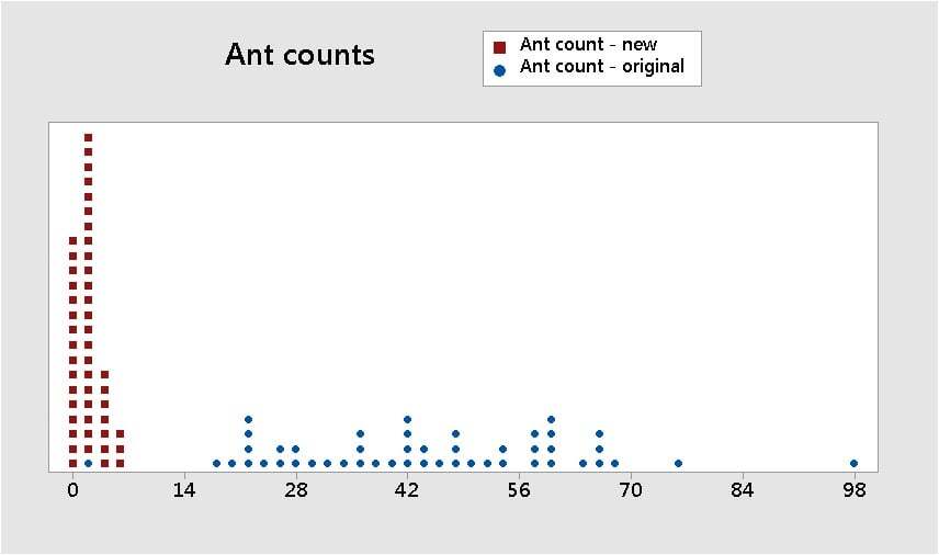
Using Poisson regression to evaluate the data set of small ant counts (shown by the red values in the dot plot below) worked out well. We avoided all of the messy problems that arose when we tried to evaluate these data using ordinary linear regression in Part 2.
Is Poisson Regression Always a Better Choice for a Count Response?
So Poisson regression can often provide more suitable results for a count response than ordinary linear regression. But is it always a better choice?
Let's go back, full-circle, to the original ant count data set from am.stat org, shown by the blue data values in the dotplot below).
In Part I, we saw that ordinary linear regression performed well with this count data. But look what happens to the model fit statisticss when these count data are evaluated using Poisson regression:
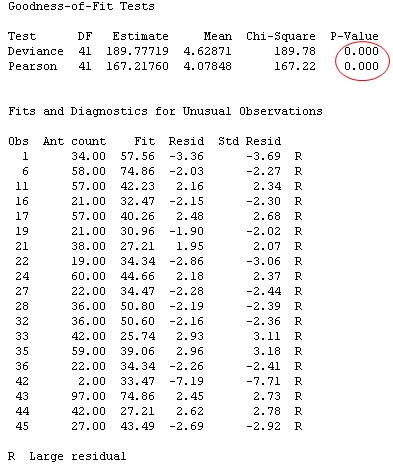
The p-value for the model fit is very small (< 0.05), indicating poor model fit. In fact, 19 of the 48 values in the data set are flagged as "unusual observations"! That's almost 40% of the data—much more than the 5% that you could expect to occur by random chance.
What's the problem?
Overdispersion: The Nemesis of a Poisson Model
One thing that can throw the proverbial wrench into a Poisson model is overdispersion. A Poisson distribution is technically defined as a distribution with equal mean and variance. If the variance of the data is much greater than its mean, it can cause problems.
For the original count data that produced all unusual observations and poor lack-of-fit results using Poisson regression, notice that the variance is nearly 8 times greater than the mean: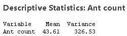
Just for illustrative purposes (never do something like this with your data!), consider what happens if you add a value of 200 to each count in this data set, to make the mean and variance closer.
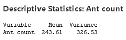
Now, if you re-run the Poisson regression analysis with this modified data, look what happens to the lack-of-fit statistics and unusual observations:
The goodness-of-fit p-values are high and indicate no evidence of lack of fit. In fact, only one data value is now flagged as an unusual observation. The Poisson model is much happier when the mean and variance are closer together (they don't have to be exactly equal, though).
Moral of the story? For the original data set of count responses, the model fit was actually better with the ordinary linear regression than it was for Poisson regression, due to overdispersion.
Sandwich Wrap Up: Analyzing a Count Response using Ordinary Linear Regression or Poisson Regression
This whole thing got started when some bored kids started throwing parts of their sandwiches to meat ants. By analyzing the ant count data in Minitab, we've seen some important issues to consider when using ordinary linear regression or Poisson regression with a count response:
| Ordinary Linear Regression | Poisson Regression |
|---|---|
|
|
Both analyses perform equally well with a ham and pickle, a peanut butter, or a Vegemite sandwich.