


About a year ago, a reader asked if I could try to explain degrees of freedom in statistics. Since then, I’ve been circling around that request very cautiously, like it’s some kind of wild beast that I’m not sure I can safely wrestle to the ground.
Degrees of freedom aren’t easy to explain. They come up in many different contexts in statistics—some advanced and complicated. In mathematics, they're technically defined as the dimension of the domain of a random vector.
But we won't get into that. Because degrees of freedom are generally not something you need to understand to perform a statistical analysis—unless you’re a research statistician, or someone studying statistical theory.
And yet, enquiring minds want to know. So for the adventurous and the curious, here are some examples that provide a basic gist of their meaning in statistics.
The Freedom to Vary
First, forget about statistics. Imagine you’re a fun-loving person who loves to wear hats. You couldn't care less what a degree of freedom is. You believe that variety is the spice of life.
Unfortunately, you have constraints. You have only 7 hats. Yet you want to wear a different hat every day of the week.

On the first day, you can wear any of the 7 hats. On the second day, you can choose from the 6 remaining hats, on day 3 you can choose from 5 hats, and so on.
When day 6 rolls around, you still have a choice between 2 hats that you haven’t worn yet that week. But after you choose your hat for day 6, you have no choice for the hat that you wear on Day 7. You must wear the one remaining hat. You had 7-1 = 6 days of “hat” freedom—in which the hat you wore could vary!
That’s kind of the idea behind degrees of freedom in statistics. Degrees of freedom are often broadly defined as the number of "observations" (pieces of information) in the data that are free to vary when estimating statistical parameters.
Degrees of Freedom: 1-Sample t test
Now imagine you're not into hats. You're into data analysis.
You have a data set with 10 values. If you’re not estimating anything, each value can take on any number, right? Each value is completely free to vary.
But suppose you want to test the population mean with a sample of 10 values, using a 1-sample t test. You now have a constraint—the estimation of the mean. What is that constraint, exactly? By definition of the mean, the following relationship must hold: The sum of all values in the data must equal n x mean, where n is the number of values in the data set.
So if a data set has 10 values, the sum of the 10 values must equal the mean x 10. If the mean of the 10 values is 3.5 (you could pick any number), this constraint requires that the sum of the 10 values must equal 10 x 3.5 = 35.
With that constraint, the first value in the data set is free to vary. Whatever value it is, it’s still possible for the sum of all 10 numbers to have a value of 35. The second value is also free to vary, because whatever value you choose, it still allows for the possibility that the sum of all the values is 35.
In fact, the first 9 values could be anything, including these two examples:
34, -8.3, -37, -92, -1, 0, 1, -22, 99
0.1, 0.2, 0.3, 0.4, 0.5, 0.6, 0.7, 0.8, 0.9
But to have all 10 values sum to 35, and have a mean of 3.5, the 10th value cannot vary. It must be a specific number:
34, -8.3, -37, -92, -1, 0, 1, -22, 99 -----> 10TH value must be 61.3
0.1, 0.2, 0.3, 0.4, 0.5, 0.6, 0.7, 0.8, 0.9 ----> 10TH value must be 30.5
Therefore, you have 10 - 1 = 9 degrees of freedom. It doesn’t matter what sample size you use, or what mean value you use—the last value in the sample is not free to vary. You end up with n - 1 degrees of freedom, where n is the sample size.
Another way to say this is that the number of degrees of freedom equals the number of "observations" minus the number of required relations among the observations (e.g., the number of parameter estimates). For a 1-sample t-test, one degree of freedom is spent estimating the mean, and the remaining n - 1 degrees of freedom estimate variability.
The degrees for freedom then define the specific t-distribution that’s used to calculate the p-values and t-values for the t-test.
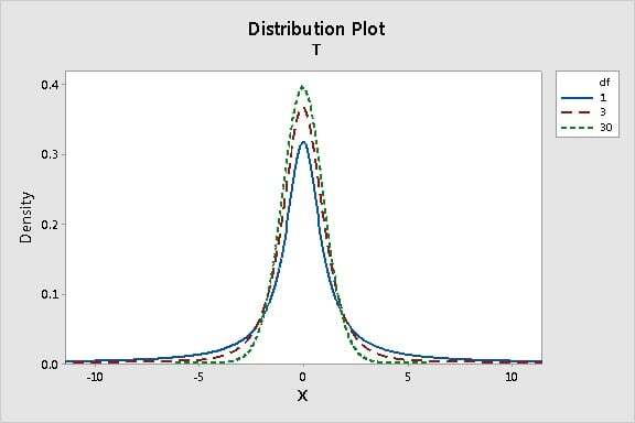
Notice that for small sample sizes (n), which correspond with smaller degrees of freedom (n - 1 for the 1-sample t test), the t-distribution has fatter tails. This is because the t distribution was specially designed to provide more conservative test results when analyzing small samples (such as in the brewing industry). As the sample size (n) increases, the number of degrees of freedom increases, and the t-distribution approaches a normal distribution.
Degrees of Freedom: Chi-Square Test of Independence
Let's look at another context. A chi-square test of independence is used to determine whether two categorical variables are dependent. For this test, the degrees of freedom are the number of cells in the two-way table of the categorical variables that can vary, given the constraints of the row and column marginal totals.So each "observation" in this case is a frequency in a cell.
Consider the simplest example: a 2 x 2 table, with two categories and two levels for each category:
|
|
Category A |
Total |
|
| Category B |
? |
|
6 |
|
|
|
15 |
|
| Total |
10 |
11 |
21 |
It doesn't matter what values you use for the row and column marginal totals. Once those values are set, there's only one cell value that can vary (here, shown with the question mark—but it could be any one of the four cells). Once you enter a number for one cell, the numbers for all the other cells are predetermined by the row and column totals. They're not free to vary. So the chi-square test for independence has only 1 degree of freedom for a 2 x 2 table.
Similarly, a 3 x 2 table has 2 degrees of freedom, because only two of the cells can vary for a given set of marginal totals.
|
|
Category A |
Total |
||
| Category B |
? |
? |
|
15 |
|
|
|
|
15 |
|
| Total |
10 |
11 |
9 |
30 |
If you experimented with different sized tables, eventually you’d find a general pattern. For a table with r rows and c columns, the number of cells that can vary is (r-1)(c-1). And that’s the formula for the degrees for freedom for the chi-square test of independence!
The degrees of freedom then define the chi-square distribution used to evaluate independence for the test.
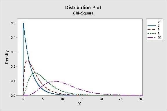
The chi-square distribution is positively skewed. As the degrees of freedom increases, it approaches the normal curve.
Degrees of Freedom: Regression
Degrees of freedom is more involved in the context of regression. Rather than risk losing the one remaining reader still reading this post (hi, Mom!), I'll cut to the chase.
Recall that degrees of freedom generally equals the number of observations (or pieces of information) minus the number of parameters estimated. When you perform regression, a parameter is estimated for every term in the model, and and each one consumes a degree of freedom. Therefore, including excessive terms in a multiple regression model reduces the degrees of freedom available to estimate the parameters' variability. In fact, if the amount of data isn't sufficient for the number of terms in your model, there may not even be enough degrees of freedom (DF) for the error term and no p-value or F-values can be calculated at all. You'll get output something like this:
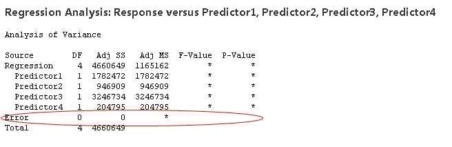
If this happens, you either need to collect more data (to increase the degrees of freedom) or drop terms from your model (to reduce the number of degrees of freedom required). So degrees of freedom does have real, tangible effects on your data analysis, despite existing in the netherworld of the domain of a random vector.
Follow-up
This post provides a basic, informal introduction to degrees of freedom in statistics. If you want to further your conceptual understanding of degrees of freedom, check out this classic paper in the Journal of Educational Psychology by Dr. Helen Walker, an associate professor of education at Columbia who was the first female president of the American Statistical Association. Another good general reference is by Pandy, S., and Bright, C. L., Social Work Research Vol 32, number 2, June 2008, available here.