


Last time I posted, I showed you how to divide a data set into training and validation samples in Minitab with the promise that next time I would show you a way to use the validation sample. Regression is a good analysis for this, because a validation data set can help you to verify that you’ve selected the best model. I’m going to use a hypothetical example so that you can see how it works when we really know the correct model to use. This will let me show you how Minitab Statistical Software’s Predict makes it easy to get the numbers that you need to evaluate your model with the training data set.
(The steps I used to set up the data appear at the end, if you want to follow along. If you do, consider skipping the steps where I set the base for the random numbers: If you produce different random numbers, the conclusion of the exercise will still be the same for almost everyone!)
Let’s say that we have some data where we know that Y = A + B + C + D + E + F + G. In regression, we usually cannot measure or identify all of the predictor variables that influence a response variable. For example, we can make a good guess about the number of points a basketball player will score in his next game based on the player's historical performance, the opponent's quality, and various other factors. But it's impossible to account for every variable that affects the number of points scored every game. For our example, we’re going to assume that the data we can collect for prediction are only A, B, C, and D. The remaining predictors, E, F, and G are real variables, but they’re going to become part of the error variation in our analysis. E, F, and G are independent of the variables that we can include in the model.
Let’s say that we collect 500 data points and decide that we can use half to train the model and half to validate the model. Then we’ll do regression on the training sample to identify some models we think are the most like the real relationship. For clarity, I'll append _1 to the variable names when I'm using the training data set, and _2 to the names when I'm using the validation data set.
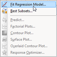 To start, I'll try fitting a model that has all the predictors that we can use in the training data set, and all of the interactions between those terms. Here's how to fit that model in Minitab Statistical Software:
- Choose Stat > Regression > Regression > Fit Regression Model.
- In Responses, enter 'Y_1'.
- In Continuous predictors, enter 'A_1'-'D_1'.
- Click Model.
- Under Predictors, highlight 'A_1', 'B_1', 'C_1', and 'D_1'.
- Under Add terms using selected predictors and model terms in Interactions through order, select 4. Click Add. Click OK twice.
Model Summary
S R-sq R-sq(adj) R-sq(pred)
1.76161 65.06% 62.82% 59.28%
This model should come close to maximizing the r2 statistic for this sample data. Once we have this model, Minitab helps out a lot. We can quickly store the predictions from the validation data set to evaluate the model.
- Choose Stat > Regression > Regression > Predict.
- In the drop-down menu, select Enter columns of values.
- In the table, enter the columns of predictors from the validation data set: 'A_2', 'B_2', 'C_2', and 'D_2'. Click OK.
The predictions for the model are now stored in the worksheet. Remember that we know that this model is wrong. No interaction effects are in the equation for the response that we defined as Y = A + B + C + D + E + F + G. Also, we know that the variables are unrelated so none of the interactions are related to the variables that we reserved for the error term.
One way to proceed is to remove terms from the model based on their statistical significance. For example, you might use the default settings with Minitab's stepwise selection procedure to find a new candidate model. Here's how to do that in Minitab:
- Choose Stat > Regression > Regression > Fit Regression Model.
- Click Stepwise.
- In Method, select Stepwise. Click OK twice.
Model Summary
S R-sq R-sq(adj) R-sq(pred)
1.75428 64.02% 63.13% 61.98%
The new model has slightly higher adjusted and predicted r2 statistics than the previous model, so it is an acceptable candidate model. This reduced model still includes two interaction terms, A_1*C_1 and B_1*C_1. So we know that this model is also wrong because we know that the real relationship doesn't include any interactions. We'll store the predictions from this model using the same steps as we did for the previous model.
Let's also do a regression with the model that we know is most like the true relationship. Here's how to quickly get that model in Minitab:
- Choose Stat > Regression > Regression > Fit Regression Model.
- Click Stepwise.
- In Method, select None. Click OK.
- Click Model.
- Click Default. Click OK twice.
Model Summary
S R-sq R-sq(adj) R-sq(pred)
1.77427 62.89% 62.28% 61.35%
Although we know that this model is the most true, the Model Summary statistics are worse than the statistics for the model that was the result of the stepwise selection. We might still use the principle of parsimony to prefer this model, but let's see what happens when we use the validation data.
Once you have the predictions stored from all 3 models, you can use different criteria to see which model fits the validation data the best, such as the predicted error sum of squares and the absolute deviations. One traditional criterion is the same one that we use to estimate the regression coefficients, minimizing the sum of the squared errors from the model. To do this in Minitab, do these steps for each model:
- Choose Calc > Calculator.
- In Store result in variable, enter an unused column.
- In Expression, enter an expression like this one: sum(('Y_2'-‘PFITS1’)^2). (In this expression, Y_2 is the name of the response column from my validation data set and PFITS1 contains the predictions from the largest model.) Click OK.
If you calculate the sums for the three models above, you get these results:
| Model |
Sum of the squared errors |
| Full model, including up to the 4-way interaction. |
812.678 |
| Stepwise model |
787.359 |
| Model with the terms from the real relationship |
774.574 |
The conclusion of the analysis, which should happen, is that the best predictions come when you try to estimate the model that’s closest to the terms in the real relationship! Because Minitab’s new Predict lets you store the predicted values from a model, you can easily compare those predictions to the real values from a validation data set. Validation can help you have more confidence in your fearless data analysis.
Steps to set up data
- Enter these column headers:
| C1 |
C2 |
C3 |
C4 |
C5 |
C6 |
C7 |
C8 |
| Y |
A |
B |
C |
D |
E |
F |
G |
- In Minitab, choose Calc > Set Base.
- In Set base of random generator to enter 1. Click OK.
- Choose Calc > Random Data > Normal.
- In Number of rows to generate, enter 500.
- In Store in column(s), enter A-G. Click OK.
- Choose Calc > Calculator.
- In Store result in variable, enter ‘Y’.
- In Expression, enter 'A'+'B'+'C'+'D'+'E'+'F'+'G'. Click OK.
- Choose Calc > Make Patterned Data > Simple Set of Numbers.
- In Store patterned data in, enter Samples.
- In From first value, enter 1.
- In To last value, enter 2.
- In Number of times to list each value, enter 250. Click OK.
- In Minitab, choose Calc > Set Base. Click OK.
- Choose Calc > Random Data > Sample From Columns.
- In Number of rows to sample, enter 500.
- In From columns, enter Samples.
- In Store samples in, enter Samples. Click OK.
- Choose Data > Unstack Columns.
- In Unstack the data in, enter Y-G.
- In Using subscripts in, enter Samples.
- Under Store unstacked data in, select After last column in use. Click OK.