


by Manikandan Jayakumar, guest blogger
In an earlier post, I discussed
how to collect data in a Design of Experiments (DOE) to optimize the value of an attribute or categorical response (Pass/Fail, Accept/Reject, etc.). I then showed how to convert the collected data into proportions and apply the arcsine transformation using built-in calculator in Minitab Statistical Software.
Now we’re ready to analyze the data to see what effect our three factors have on our attribute response!
Initial Model and Interaction Plot of Attribute DOE Results
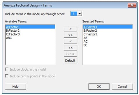
We’ll do this by choosing Stat > DOE > Factorial > Analyze Factorial Design…. Choose the arcsine-transformed proportions as the Response, then click terms and select the main factors and two-way interactions:
The P-values in the table below indicate that interactions between the factors are not significant.
We can use Minitab’s Interactions Plot to visualize what these data are telling us. An interactions plot is a plot of means for each level of a factor with the level of a second factor held constant. Interaction is present when the lines intersect each other. Minitab can create a single interaction plot for two factors, or a matrix of interaction plots for three to nine factors.
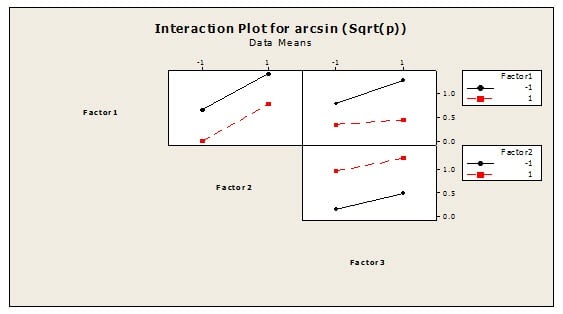
The lines in the interaction plot do not intersect each other, which indicates there is no interaction between the factors. This is consistent with what we observed in the p-values for the interactions.
Analyzing the Attribute Response DOE with a Reduced Model
Since we know that the interactions between the factors are not significant, we can remove them from our model and rerun the analysis using only our three main factors. Once again, we’ll choose Stat > DOE > Factorial > Analyze Factorial Design… and choose the arcsine-transformed proportions as the Response. But this time, when we enter the terms in our model, we include only the three main factors.
The output is shown below.
The p-values indicates Factor1 and Factor2 are significant, but not Factor3.
Main Effects Plot of Attribute DOE Results
We can visualize these results with a Main Effects Plot. A “main effect” is present when different levels of a factor affect the response differently. A Main Effects Plot is used in conjunction with ANOVA and DOE to examine differences among level means for one or more factors.
A Main Effects Plot graphs the response mean for each factor level, connected by a line. When the connecting line is horizontal (parallel to the x-axis), no main effect exists—each level of the factor affects the response in the same way, and the response mean is the same across all factor levels. When the line is not horizontal, different levels of the factor affect the response differently. The less horizontal the line, the greater the likelihood that a main effect is statistically significant.
Here are the Main Effects Plots for our data:
The Main effect is present in Factor1 and Factor2 as the lines are vertical. In this example, “Larger is better,” so we can conclude we want to set the levels to -1 for Factor1 and +1 for Factor2. Since “Factor 3” is not statistically significant, the level for Factor 3 will not significantly influence the desired outcome. We can therefore remove Factor 3 from the model.
Using the Response Optimizer
The Response Optimizer in Minitab helps to identify the combination of input variable settings that jointly optimize a single response or a set of responses. It gives you an optimal solution for the input variable combinations, along with an optimization plot. The optimization plot is interactive—you can adjust input variable settings on the plot to search for more desirable solutions
Using the Response Optimizer, we find that the maximum response (arcsin) is 1.4179, with a desirability of 1.
Final Solution
The analysis has shown that parameters for factors are set at the following levels to achieve the maximum attribute response:
Factor 1 --> -1
Factor 2 --> +1
Factor 3 --> +1 (Factor 3 is insignificant and might not create high impact if it is changed to -1)
Back Transformations
As a final step, the transformed arcsine data may be converted back into percentages with the inverse function:
P = (sin arcsin (sqrt(P))2
The diagram below shows the relationship between the arcsin and Proportion. It indicates there is nonlinear relationship between them.
In the Response Optimizer, we found that setting Factor 1 to the low level and Factor 2 to the high level produces an arcsin value of
1.57 with a desirability of 1. The value 1.57 is therefore the optimum value since a desirability of 1 is the maximum you can obtain. But a high increase or decrease in the arcsin value might affect the proportion, as the relationship is nonlinear.
To verify the optimized factor settings, 30 experiments were conducted. The attribute response was positive for all 30 experiments. Based on the results, the new process settings were approved and updated in all the appropriate process documents.
About the Guest Blogger:
Manikandan Jayakumar is a Lean Six Sigma specialist with over 8 years’ experience in process improvement across the automotive, software and service industries. He currently works in Six Sigma deployment with organizations in India. He has trained over 300 candidates in Lean Six Sigma and mentored more than 80 Green and Black Belts along the way. He is a certified Black Belt and a Master Black Belt Candidate from Visteon and the Indian Statistical Institute.
If you would like to be a guest blogger on the Minitab Blog, contact publicrelations@minitab.com.