This is part two in a series. Read part one here.
In part 1, I used Minitab Statistical Software to develop a regression model that describes the relationship between body mass index (BMI) and body fat percentage. In this post, I will use this model to predict body fat percentage and assess the precision of my predictions. I'll also compare Minitab's predictions to those of bathroom scales that use bioelectrical impedance analysis (BIA) to estimate percent body fat.
Assessing Predicted R-Squared
Previously, I used a Fitted Line Plot to assess the model. To generate predictions, I’ll use the same model, but I need to use General Regression. General Regression gives us an additional piece of output that is crucial for prediction, the predicted R-squared. The predicted R-squared indicates how well the model predicts new observations. Here’s the Summary of Model table from General Regression.

For our model, the predicted R-squared is 74.14%. Because this value is close to the R-squared of 76.06%, the model provides valid predictions.
However, in the case of a model where the regular R-squared is good but the predicted R-squared is significantly lower, it indicates that the model fits the original data but fails to provide valid predictions. This tends to happen when the model is overly complicated and it starts to model the noise in the data. This condition is known as "overfitting the model." Be sure to check the predicted R-squared before making predictions!
Regression Prediction Constraints
Let's review several important considerations before we start. First, regression predictions are valid only for the range that the original data covers. So, we should generate predictions only for BMI values between 15 and 35. Predictions are also valid only for the population that the data represents. In this case, the population is females between the ages of 12 to 14 years.
We only know the relationship between BMI and fat percentage within this data range and for this population. Outside of these conditions, the shape of the curve could change, which would throw our predictions off. In other words, we just don't know beyond what we actually measure.
Making a Prediction with General Regression
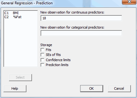
We have a good model with a good predicted R-squared. So, we're ready to make a prediction! In Minitab, I choose Stat > Regression > General Regression... then fill out the Prediction dialog like this to predict the percent of body fat for a BMI of 18:

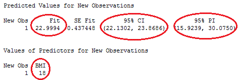
We get the following output:

For a BMI of 18, the predicted (or fitted) value of fat percentage is ~23%. But, how precise is this prediction? Minitab provides two measures:
The prediction interval (PI) represents the range that a single new observation is likely to fall within. So, we can be 95% confident that a specific person's body fat will fall between 16% and 30% (or +/- 7%) if her BMI is 18.
The confidence interval (CI) represents the range that the mean value is likely to fall within. We can be 95% confident that the mean body fat percentage for all girls in this age group, who have a BMI of 18, will fall between 22.1% and 23.9% (or approximately +/- 1%).
The prediction interval is always wider than the corresponding confidence interval because of the added uncertainty involved in predicting a single value versus the mean value.
Comparing Minitab Predictions to BIA Scale Estimates
The percentage of body fat as measured by the DXA machine is the true and accurate health measure. Both the BMI regression analysis and the BIA scales try to estimate the percentage of body fat. Let’s see how the accuracy and precision of the regression predictions compare to those from BIA scales.
To use these scales, you enter your gender and height, and the scale measures your weight. It also sends a low electrical current through your body to estimate the fat mass. I didn’t measure the subjects on these scales because this was not part of the project. However, I checked several Web sites (here and here) that interviewed experts in energy metabolism and exercise about these scales. I found several ways to compare the two methods. The bold statements are about errors in the readings from BIA scales followed by a comparison to the Minitab predictions.
The scales produce estimates that have larger errors for the extremely lean or obese.
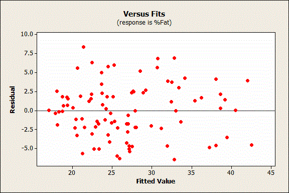
This problem is called nonconstant variance, or heteroscedasticity. Minitab's predictions based on this model don’t have this problem. In fact, we always check for this condition while fitting a regression model using the residual plots. To check for heteroscedasticity, we look at the residuals versus fits plot (below). We can see whether the residuals fan out at the higher and/or lower ends of the range. However, in the plot below, we see a constant spread (or variance) around zero, which indicates the preferred homoscedasticity.

The scales tend to overestimate percent body fat in very lean individuals and underestimate body fat in obese people.
Systematic errors like this are known as bias. Minitab's predictions based on this model don’t have this problem. This is another condition that we always assess while fitting regression models. To assess this, we again look at the residuals versus fit plot (above). If our model produces the same bias as the scales, we’d see a pattern in the residuals. The plot would show more positive residuals on the left and more negative residuals on the right. Instead, we see residuals that are randomly above and below throughout the range, which indicates no bias.
The scales produce estimates of the true fat percentage that can be off by +/- 5%.
We found that our regression model produced predictions that can be off by +/- 7% for an individual. One big caveat here: we know that the Minitab predictions have a 95% confidence of being within this interval, but I could not find the confidence level for the estimates produced by the bathroom scales. However, the size of the intervals are in the same ballpark. I’m calling this a tie.
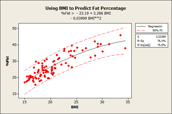
I've plotted the prediction interval in the Fitted Line Plot below to show that the width of the prediction interval remains nearly constant over the full range of the data.

The scales produce estimates that can be wildly unstable unless you follow a rigid protocol. You must use the scale at a constant level of hydration, a fixed time of day, and a fixed point in the menstrual cycle. You also can't exercise or shower in the hours before the measurement.
The Minitab predictions don’t have this stability problem because they clearly don’t depend on these factors. A BMI of 18 will always produce the same estimate with this model. Further, the predictions should be valid because the predicted R-squared is nearly equal to the R-squared.
Closing Thoughts About Prediction with Regression
Both methods incorporate your height, weight, gender, and age (our model is for middle-school girls). BIA scales add the electrical signal and, honestly, I don’t see that it adds anything other than noise to their results! In the best-case scenario where someone follows the rigid BIA scale protocols and is not unusually lean or obese, both the BMIs and the scales produce predictions with similar-sized prediction intervals. However, as you move toward extreme values or stop following the rigid protocol, the electrical signals produce erratic results and Minitab's predictions start to win out.
However, before we rush out to sell our model as a replacement for these scales, keep in mind that our model applies only to middle-school aged girls. There’s a lot of work to be done to apply it to males and to different age groups. What we’ve done amounts to a pilot study that demonstrates the feasibility of the approach.
If you're learning about regression, read my regression tutorial!


