


Previously in our designed experiment on driving the golf ball as far as possible from the tee, we tested our four experimental factors and determined how many runs we needed to produce a complete data set.
Now let’s analyze the data and interpret the covariates and blocking variables.
For each drive, we recorded the experimental factor settings, club speed, club / ball contact efficiency, and the golfer. Our analysis will focus first on removing the effect of the last three noise variables from the data so that we can get a clearer look at our 4 research variables.
Analysis of Covariance (ANCOVA)
A covariate is a continuous noise variable that has an impact on your response, but is not of research interest. Analysis of covariance removes the impact of covariates from the data so you can determine the effects of the experimental factors. Two quick examples:
- When comparing the weight loss from two diet plans, the % body fat of each subject at the start of the experiment is a covariate because the pounds lost will be higher for those with a high initial % body fat for both diet plans.
- When studying the effects of process settings of a water treatment for removing solids from waste water, the turbidity (cloudiness) of the treated water will be a function of the incoming water turbidity regardless of the treatment process.
Consider the scatterplot below, which shows two golfers’ Carry distance vs the club speed for that drive. There is a great deal of variability in the response around the regression line because of the variety of experimental factor settings used for each drive. Still, the impact of the club speed can be seen within this variability. The regression line for the impact of the club speed is:
Carry (yd) = 109 + 1.055 * (Club Speed in mph)
The average club speed is 89.6 mph. Essentially, ANCOVA adjusts each data point down about 1.055 yards for each mph the club speed is above 89.6 mph and adjusts up for data points below the average of 89.6 mph.
The final experiment analysis will be on the adjusted data points, not the original Carry values. By doing this, we can measure the effects of our four input variables while controlling for club speed and club / ball contact efficiency, our two covariates.

I have used ANCOVA to study the effects of process parameter settings on the final flatness of silicon disks from a machining process, while controlling for the flatness of the blanks coming into the process. I have also used ANCOVA to learn the effects of curriculum characteristics on the test scores of high school students, while controlling for the students’ past academic performance and years of schooling of their parents. It is a powerful technique that allows us to make apples-to-apples comparisons with data that would otherwise bias the results.
This analysis can be done in Minitab by double-clicking the appropriate column(s) into the Covariate dialog box..
Blocking Variables
A blocking variable is a categorical noise variable that affects your response but is not of research interest. This dotplot compares the Carry distance of each of the four golfers in our study. It shows a great deal of golfer-to-golfer variability even though they each tested equivalent settings of all four experimental factors. How are we going to combine this data and analyze it as one experiment? The answer is simple — blocking.

We designed our data collection to block on golfer to ensure that each golfer would be testing equivalent combinations of the four factors. This is called balance. Based on this design, Minitab will also know to include golfer in the analysis.
See how your company can learn to effectively utilize data to make smarter decisions. Learn more about our Training Services today!
There are four key benefits to blocking in your experiment design:
1. All the data will be standardized.
The effect of the blocking variable at each level (in this case, our four golfers) will be estimated by the average response at that level. This standardization essentially removes the effect of the blocking variable so that all the data can be analyzed as one experiment. This is similar to analysis of covariance, the major difference being that the data collection can be designed to be balanced with respect to the blocking variable, whereas this isn’t always possible with covariate(s).
2. Blocking allows you to complete the data collection more efficiently.
All resources (3 machines, 4 batches, 2 gages, etc.) are used without concern over adding variability to your results. The variability will be accounted for by attributing it to the blocking variable, thus preventing it from negatively affecting your results.
3. Your results will be applicable over a wider range of conditions.
Our results will apply to the range of golfers’ styles and abilities. We will also learn the relative importance of the blocking variable compared to the research variables. I saw this benefit benefit of blocking when I was working with a manufacturer of ultrasonic transducers who was having difficulty meeting a flatness specification, a key quality characteristic. We decided to run a 3-factor full factorial on each of the three production machines instead of just one. In the end, we found the three process variables had no effect on flatness: only one of the machines was causing the poor flatness results because of a fixture issue. Good thing we decided to block!
4. Blocking accounts for the variability caused by the blocking variable.
This reduces the error term used in all hypothesis tests and thus increases their power to detect a significant effect. Consider this ANOVA table comparing the cure time for three polymer formulations tested over several batches of raw material.
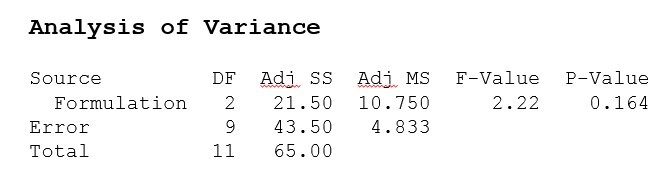
The p-value for the F-test comparing the three formulations is 0.164, which means this test failed to detect that one of the formulations is different. This is based on an average error estimate that includes the batch-to-batch variation. If the batch-to-batch variation is separated from the error estimate by including the blocking variable (Batch) in the analysis, here is the resulting ANOVA table.

The p-value for the F-test comparing the three formulations is now 0.031, so we reject the null hypothesis that all three formulations have the same mean cure time and conclude that at least one formulation is different. We also learn that the batch-to-batch variation has roughly the same impact on cure time as the formulations we were studying.
I hope I've made a strong case for the importance of including a blocking variable in the design and analysis of your DOE. Many a designed experiment has been made or broken based on the researcher’s planning for categorical noise variable(s) that would impact their response.
The two covariates, club speed and club / ball contact efficiency, as well as the blocking variable (Golfer), will be included in our final analysis, giving us a clearer assessment of the effects of our four experimental factors on our response, Carry distance. Next time we’ll review the results!
Take your data to the next level with Minitab.

Many thanks to Toftrees Golf Resort and Tussey Mountain for use of their facilities to conduct our golf experiment.
Catch Up with the other Golf DOE Posts:
Part 1: A (Golf) Course in Design of Experiments
Part 2: 5 Reasons Factorial Experiments Are So Successful
Part 3: Mulligan? How Many Runs Do You Need to Produce a Complete Data Set?
Part 5: Concluding Our Golf DOE: Time to Quantify, Understand and Optimize