


In my last post, I discussed how a DOE was chosen to optimize a chemical-mechanical polishing process in the microelectronics industry. This important process improved the plant's final manufacturing yields. We selected an experimental design that let us study the effects of six process parameters in 16 runs.
Analyzing the Design
Now we'll examine the analysis of the DOE results after the actual tests have been performed. Our objective is to minimize the amount of variability (minimize the Std Dev response) to achieve better wafer uniformity. At the same time we would like to minimize cycle times by increasing the Removal Rate of the process (maximize the V A°/Min response).
Therefore, we are dealing with a multi-response DOE.

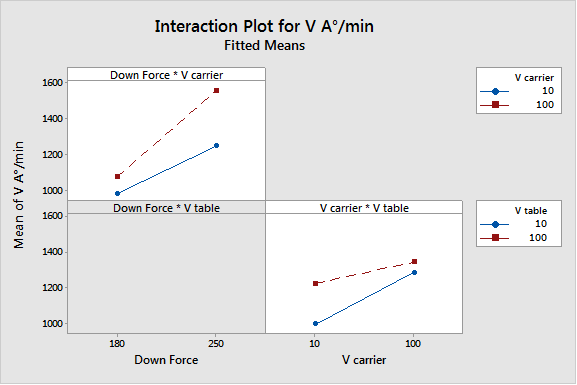
From the DOE data shown above, we first built a model for the Removal Rate (V A°/Min): Down Force, Carrier velocity and Table velocity had a significant effect, as the Pareto chart below clearly shows. The Down Force*Carrier velocity and the Carrier velocity*Table velocity two-factor interactions were also significant. We therefore eliminated the remaining parameters, which were not significant, from the model, gradually.

A process expert later confirmed that such effects and interactions were logical and could have been expected from our current knowledge of this process. The graph below shows the main effect plots (Removal Rate response).

We had chosen a fractional DOE, so several two-factor interactions were confounded with one another. However, the Down Force*Carrier velocity and the Carrier velocity*Table velocity interactions made more sense from a process point of view; besides, these two interactions were associated with very significant main effects.
We built a second model for the standard deviation response. The standard deviation does not necessarily follow a normal distribution, therefore a log transformation is needed to transform Standard deviation data into normality.
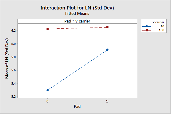
Carrier velocity, Pad and Table velocity as well as the Pad*Carrier velocity interaction had significant effects on the logarithm of the Standard deviation response, as shown in the Pareto graph below. Again this was quite logical and confirmed our process knowledge.

The main factor effects are shown in the graph below (Log of Standard Deviation).

The interaction effect is shown in the graph below (Logarithm of Standard Deviation response).
We then compared the predictions from our two models to the real observations from the tests, in order to assess the validity of our model. We were interested in identifying observations that would not be consistent with our models. Outliers due to changes in the process environment during the tests often occur, and may bias statistical analyses.
The residual plots below represent the differences between real experiment values and predictions based on the model. Minitab provides four different ways to look at the residuals, in order to help assess whether these residuals are normally and randomly distributed.

In these diagrams, the residuals seem to be generally random (shown by the right hand plots, which display the residuals against their fitted values and their observation order) and normally distributed (displayed by the probability plot on the left).
But the observation in row 16 (the blue point that has been selected and brushed in the plot below) looks suspicious as far as the residuals for the removal rate (V A°) response are concerned. It is positioned farther away from the other residual values. We used the brushing functionality in Minitab to get more information about this point (see the values in the table below). We then eliminated observation number 16, and reran the DOE analysis...but the final Removal Rate model was still very similar to the initial one.

From our two final models, we used the process optimization tool within Minitab to identify a global process optimum. Two terms were included in the Standard Deviation model (V Carrier: E, Pad: D, and V Table: F), and three terms plus some interactions were included in the Removal Rate (V A°) model (Down Force: A, V Carrier: E and V Table: F).
Finding the best compromise while considering conflicting objectives is not always easy, especially when different models contain the same parameters. Reducing the standard deviation to improve yields was more important than minimizing cycle times. Therefore, in the Minitab optimization tool, we assigned a score of 3 in terms of importance to the standard deviation response and a score of only 1 to the V A° (Removal Rate) response.
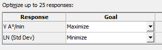


The Minitab Optimization Tool results indicate that the Down Force needs to be maximized to increase the Removal Rate (reduce Cycle time), whereas Carrier and Table velocities as well as Pad need to be kept low in order to achieve a smoother, uniform surface (a small standard deviation).
Confirmation tests run at the settings recommended by the optimization tool were consistent with the conclusions that had been drawn from the DOE.
Conclusion
This DOE proved to be a very effective method to identify the factors that had real effects by making them clearly emerge from the surrounding process noise. This analysis thus gave us both a very pragmatic and accurate approach to adjusting and optimizing the polishing process. The conclusions from the DOE could easily be extended to the operating process.