


You might be thinking, six weeks and you’re still not telling us what happened? When you are solving a manufacturing or development problem you might hear the same thing from your leadership – when will we get the results?
Never fear, we are right on schedule. According to Design and Analysis of Experiments author Doug Montgomery, “If you have 10 weeks, eight of them should be spent planning and designing the data collection, one week to execute the experiment, and one week to analyze the results.”
That’s the schedule our experiment followed, only it’s not going to take us a week to analyze. With Minitab, I rarely spend more than a day!
Last week we reviewed analysis of covariance and blocking variables in our ongoing DOE on how to get the longest drive in your golf game. Now let’s finish it. We’re ready to review and present our results.
In my experience, the researcher has three typical goals — quantify, understand and optimize. Different projects will prioritize these three goals differently, emphasizing one or another, but we are typically interested in all three.
Quantify using ANOVA
Analysis of variance was used to develop a model for Carry distance as function of our 4 experimental variables and their 6 potential two-way interactions. Let’s focus first on our two fastest-swinging golfers because their swing characteristics were very similar. After removing insignificant terms, the ANOVA table and resulting equation can be seen below for the reduced model:

The ANOVA table above highlights a few concepts we noted last week. We see the two covariates are statistically significant and to account for this, each drive has been adjusted for the club speed and club/ball contact efficiency. On the other hand, between our two highest swing-speed golfers – Sean and Andy – there is no real block effect as indicated by the high p-value = .478. We also see that by including each of those variables in the analysis, the sum of squares variation associated with those three noise variables are accounted for in the ANOVA table and that variability does not end up in the unexplained variation at the bottom of the table called Error. This reduces the error term in our F-tests for the significance of each effect, which then increases the power of the test.
The ANOVA table also points to some of the stronger effects within the list of statistically significant effects. This is indicated by the size of the F statistic, which is the ratio of the effect size to the error variation. The larger F statistic for the main effect of Ball (18.01) and the Tilt by Shaft interaction (21.94), indicate these are two of the dominant effects on Carry distance.
The regression equation quantifies each effect so that the golfer can make a good decision on which drive settings they will incorporate in their game. For example, the coefficient for Ball Characteristics is 3.75, which means that the difference in yardage between the economy ($20 / dozen) and expensive ($50 / dozen) level of Ball is 3.75 x 2 = 7.5 yards. In short, our golfers have a business decision to make: whether to spend $30 for an average improvement of 7.5 yards greater drive distance. This will make good sense for some golfers and won’t for others, but once you quantify the effects, you have the information you need to make the right business decision for your situation.
In an industrial setting, you might find that a more expensive welding rod and slower weld travel produces a stronger metal bond. Based on your regression equation, you can make a good business decision about the cost for the welding rods and how many fewer parts per hour you will produce in exchange for the improvement in weld strength needed to meet your customer’s specifications. Everyone’s process is different, but quantifying the effects of process variables with your regression equation(s) allows you to determine the settings needed to improve your process in order to meet your customer’s specifications.
Understand Using an Interaction Plot
From a first principles perspective, it is important to understand why the regression coefficients and the effects turned out the way they did. Our expanded understanding of the process allows us to move to new variable settings, which improve process results. It also informs us about other variables we need to control to consistently maintain that improved performance. Consider the Club Face Tilt * Shaft Stiffness interaction, a key contributor to Carry distance, shown in the interaction plot below:
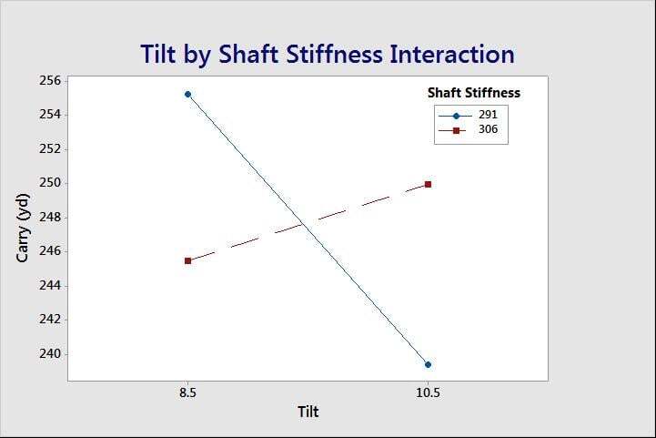
The plot shows that at a high club face tilt (10.5 degree), Carry improves if the club shaft is stiff at 306 vibrations per cycle, but the higher tilt causes a decrease in Carry if the less stiff shaft is used. This makes sense when we remember that Andy and Sean were our two highest club-speed golfers. As club velocity increases, the shaft bends away from the ball, and this changes the angle the club face presents to the ball at the bottom of the swing, independent of the tilt built into the club face. So we should expect that these two factors would interact.
Our experiment demonstrates the impact of this phenomenon on Carry distance and helps us better understand the first principle’s science behind getting that ball to travel further. Based on this understanding, perhaps we would benefit from an even stiffer shaft and higher club face tilt, or an even lower stiffness and lower club face tilt.
Understanding your process is key. I recall experimenting with a glass grinding operation in an effort to increase the glass removal rate while maintaining a smooth glass finish. We studied grit size, part rpm, grinding wheel velocity, grinding pressure, and grinding media density. Everyone was surprised to learn that the surface finish quality was only a function of grit size, which left us with complete freedom to maximize glass removal by focusing on the other four process parameters. Our improved understanding of the process led the way to us meeting our goals.
Optimization with a Cube Plot
The response optimizer and contour plot are two of my favorite tools for finding the optimal process settings. However, we only have one response and four important factors to consider, so in this case I think the cube plot fits the job. A cube plot of the average Carry at all 16 combinations of our 4 experimental factors is shown below.
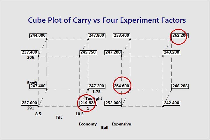
Based on this straightforward representation of the data, we can determine the conditions that produced the lowest and the highest response:
Ball = Economy, Tee Height = 1, Tilt = 10.5, Shaft = 291 ……………. Carry = 220 yards
Ball = Expensive, Tee Height = 1.75, Tilt = 8.5, Shaft = 291 ………… Carry = 265 yards
Ball = Expensive, Tee Height = 1.75, Tilt = 10.5, Shaft = 306 ……….. Carry = 262 yards
Based on these results, we conclude that we can improve our performance up to a maximum of 45 yards (20%) with an average improvement of 20 yards (8.2%). This is achieved by just using the process settings that have been optimized based on our experiment results, as opposed to the old way of driving off the tee.
Now I have a quick question for you: What would be the dollar value to your company if the process you are working on started to produce 8% more product each day, just by changing the process parameter settings?
Wrapping Up and Future Direction
In wrapping up, we need to remember the impact of noise variables in our experiment. The scatterplot of Carry distance vs. Club Speed, Club/Ball Contact Efficiency, and Golfer shown below reminds us of what we already knew. The noise variables dominate the response.
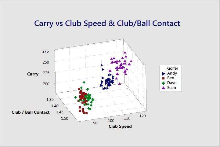
Luckily, the results of our experiment are independent of noise variables. The results are the conditions that maximize drive distance given the fact that club speed might be limited to an average of about 90 mph.
Often our results don’t guarantee a certain response level, but allow us to do the best we can with a poor raw material supply, a humid day, a dull cutting tool, etc. This will be in addition to running optimally when the noise variables are more favorable as well. So what’s next? Even though we have reached a very positive endpoint, there are still some unanswered questions. What is the effect of ball spin? Can we move to even better factor settings? What about club weight?
Most good experiments lead to even more good experiments. Until next time!
Many thanks to Toftrees Golf Resort and Tussey Mountain for use of their facilities to conduct our golf experiment.
Catch Up with the Previous Golf DOE Posts:
Part 1: A (Golf) Course in Design of Experiments
Part 2: 5 Reasons Factorial Experiments Are So Successful
Part 3: Mulligan? How Many Runs Do You Need to Produce a Complete Data Set?
Part 4: ANCOVA and Blocking: 2 Vital Parts to DOE