The Empirical CDF, Part 1: What's a CDF?

T'was the season for toys recently, and Christmas day found me playing around with a classic, the Etch-a-Sketch. As I noodled with the knobs, I had a sudden flash of recognition: my drawing reminded me of the Empirical CDF Plot in Minitab Statistical Software. Did you just ask, "What's a CDF plot? And what's so empirical about it?" Both very good questions. Let's start with the first, and we'll save that second question for a future post.

The acronym CDF stands for Cumulative Distribution Function. If, like me, you're a big fan of failures, then you might be familiar with the cumulative failure plot that you can create with some Reliability/Survival tools in Minitab. (For an entertaining and offbeat example, check out this excellent post, What I Learned from Treating Childbirth as a Failure.) The cumulative failure plot is a CDF.

Even if you're not a fan of failure plots and CDFs, you're likely very familiar with the CDF's famous cousin, the PDF or Probability Density Function. The classic "bell curve" is no more (and no less) than a PDF of a normal distribution.

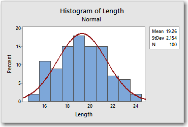
For example, here's a histogram with a fitted normal PDF for PinLength.MTW, from Minitab's online Data Set Library.

To create this plot, do the following:

1. Download the data file, PinLength.MTW, and open it in Minitab.
2. Choose Graph > Histogram > With Fit, and click OK.
3. In Graph variables, enter Length.
4. Click the Scale button.
5. On the Y-Scale Type tab, choose Percent.
6. Click OK in each dialog box.

The data are from a sample of 100 connector pins. The histogram and fitted line show that the lengths of the pins (shown on the x-axis) roughly follow a normal distribution with a mean of 19.26 and a standard deviation of 2.154. You can get the specifics for each bin of the histogram by hovering over the corresponding bar.

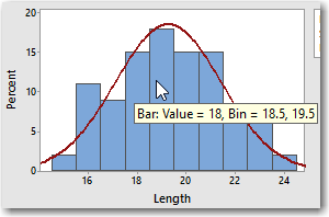
The height of each bar represents the percentage of observations in the sample that fall within the specified lengths. For example, the fifth bar is the tallest. Hovering over the fifth bar reveals that 18% of the bins have lengths that fall between 18.5 mm to 19.5 mm. Remember that for a moment.

Now let's try something a little different.

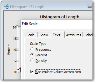
1. Double-click the y-axis.
2. On the Type tab, select Accumulate values across bins.
3. Click OK.

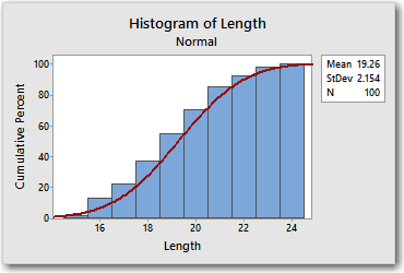
It looks very different, but it's the exact same data. The difference is that the bar heights now represent cumulative percentages. In other words, each bar represents the percentage of pins with the specified lengths or smaller.

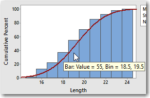
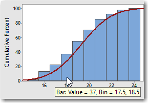
For example, the height of the fifth bar indicates that 55% of the pin lengths are less than 19.5 mm. The height of the fourth bar indicates that 37% of pin lengths are 18.5 or less. The difference in height between the 2 bars is 18, which tells us that 18% of the pins have lengths between 18.5 and 19.5. Which, if you remember, we already knew from our first graph. So the cumulative bars look different, but it's just another way of conveying the same information.

You may have also noticed that the fitted line no longer looks like a bell curve. That's because when we changed to a cumulative y-axis, Minitab changed the fitted line from a PDF to... you guessed it, a cumulative distribution function (CDF). Like the cumulative bars, the cumulative distribution function represents the cumulative percentage of observations that have values less than or equal to X. Basically, the CDF of a distribution gives us the cumulative probabilities from the PDF of the same distribution.

I'll show you what I mean. Choose Graph > Probability Distribution Plot > View Probability, and click OK. Then enter the parameters and x-value as shown here, and click OK.

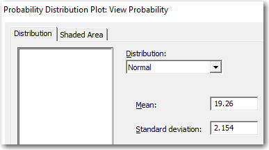
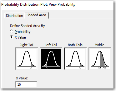
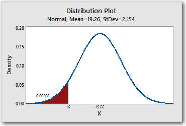
The "Left Tail" probabilities are cumulative probabilities. The plot tells us that the probability of obtaining a random value that is less than or equal to 16 is about 0.065. That's another way of saying that 6.5% of the values in this hypothetical population are less than or equal to 16.

Now we can create a CDF using the same parameters:

1. Choose Graph > Empirical CDF > Single and click OK.
2. In Graph variables, enter Length.
3. Click the Distribution button.
4. On the Data Display tab, select Distribution fit only.
5. Click OK, then click the Scale button.
6. On the Percentile Lines tab, under Show percentile lines at data values, enter 16.

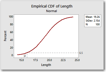
The CDF tells us that 6.5% of the values in this distribution are less than or equal to 16, as did the PDF.

Let's try another. Double-click the shaded area on the PDF and change x to 19.26, which is the mean of the distribution.

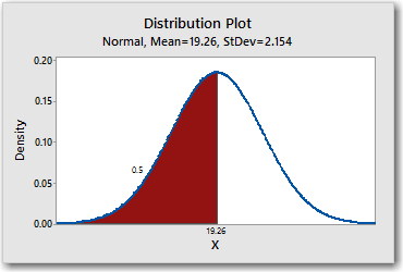
Naturally, because we're dealing with a perfect theoretical normal distribution here, half of the values in the hypothetical population are less than or equal to the mean. You can also visualize this on the CDF by adding another percentile line. Click the CDF and choose Editor > Add > Percentile Lines. Then enter 19.26 under Show percentile lines at data values.

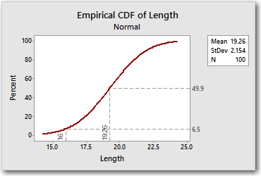
There's a little bit of rounding error, but the CDF tells us the same thing that we learned from the PDF, namely that 50% of the values in the distribution are less than or equal to the mean.

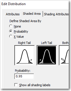
Finally, let's input a probability and determine the associated x-value. Double-click the shaded area on the PDF, but this time enter a probability of 0.95 as shown:

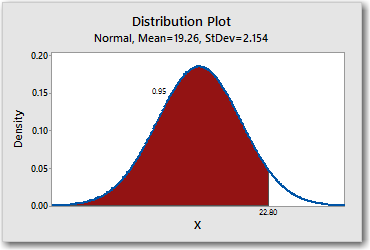
The PDF shows that the x-value that is associated with a cumulative probability of 0.5 is 22.80. Now right-click the CDF and choose Add > Percentile Lines. This time, under Show percentile lines at Y values, enter 95 for 95%.  

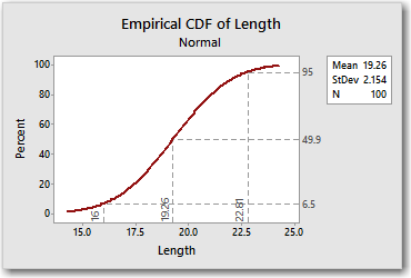
Once again, other than a little rounding error, the CDF tells us the same thing as the PDF.

For most people (maybe everyone?), the PDF is an easier way to visualize the shape of a distribution. But the nice thing about the CDF is that there's no need to look up probabilities for each x-value individually: all of the x-values in the distribution and the associated cumulative probabilities are right there on the curve.