I want to offer some clarification on my earlier blog about Cluster Analysis.
There may have been some confusion as to what the four dendrograms were trying to display in my prior post. The first dendrogram in the four-graph layout represented the final partition if the user chose only one cluster. If the user chose the final partition to be four clusters, the end result would be the last graph in the layout. The four graphs were trying to illustrate which clusters (distinguished by color) Minitab sequentially chooses as you increase the value of the final partition from 1 to 4.
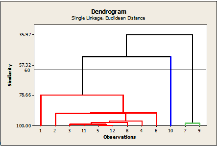
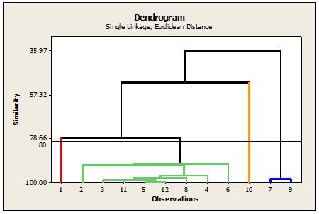
The alternative to selecting the number of clusters as the final partition is to select similarity level. Imagine a horizontal line at a similarity level equal to ‘X’ on your dendrogram. Then look at any vertical lines that intersect with your imagined line at X. If one vertical line below X goes straight down to 100%, it’s a cluster. If another vertical line goes down to another group of other observations (which are represented as smaller vertical lines on the graph), then that entire group is a cluster. Here are some examples of similarity levels set at different values of X for a more visual explanation.
X=50 (two final clusters…red and green):
X= 60 (three final clusters…red, blue, green) 
X= 80 (four final clusters…red, green, yellow, blue)
When going through the Multivariate menu within Minitab, you will see three items that pertain to Clustering:
• Cluster Observations
• Cluster Variables
• Cluster K-Means
Cluster Observations and Cluster Variables are hierarchical clustering methods, discussed in Part 1, where you start with individual clusters which are then fused to form larger clusters. Which one should you choose? Well, if you want to consider each row of your worksheet as a group to be clustered, then go with Cluster Observations. If you want to consider each column as a group, then choose Cluster Variables.
Cluster K-Means is similar to Cluster Observations as it also assumes that each row of the data set is considered a group, waiting to be classified into smaller clusters. If you have 143 rows in your worksheet, these are 143 items that eventually will be organized. There is a twist, however: unlike hierarchical clustering, it is possible for two clusters to be split into separate clusters after they are joined together.
K-Means procedures work best, though, when you provide good starting points for cluster forming. A “starting point” is a row in the worksheet that you select to be representative of a group that you have in mind. Our Example for Cluster K-Means in Minitab Help does a good job of running through how to set up these starting points in your worksheet. The Example talks about 143 bears that need to be classified based on characteristics such as height, weight, and neck girth. The user wants to classify these 143 bears into three clusters: small, medium, large. Thus, the user needs three starting points, one for each of these bear sizes. An indicator column can be created in the worksheet so that the row that represents characteristics of a small bear can get a value of 1. For the row that represents characteristics of a medium bear, you can set a value of 2, and 3 for a large bear. For all other rows that are not used as starting points, the value can be set to 0.
When you open up the dialog box for Cluster K-Means you will see that you can either specify a number of clusters or supply an initial partition column that contains group codes. For the prior example, you would electing to use an initial partition column.
I hope this information helps when running a Cluster Analysis, and hope that any prior questions were clarified from this post!


