


Minitab 17.2 is available. You can check out all of the new stuff on the What’s New Page, but I would say that a little demonstration is in order. Here are some new shortcuts that make arranging your data easier in Minitab 17.2.
Sorting
Let’s suppose that you had copied some Human Development Index data into Minitab and wanted to sort countries in the order of their rank. In the past, you would have used the Data menu, identified all the columns that you wanted to sort, selected the column that you wanted to sort by, and then selected where to store the sorted columns. In Minitab 17.2, you can do all those steps faster with a right-click:
- Select a cell in HDI Rank.
- Right-click and choose Sort Columns > Entire Worksheet > Smallest to Largest.
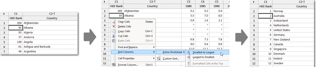
That’s it, you’re done! If your column is text, you can select whether to sort alphabetically or reverse alphabetically instead of by increasing or decreasing numeric values.
Changing data format
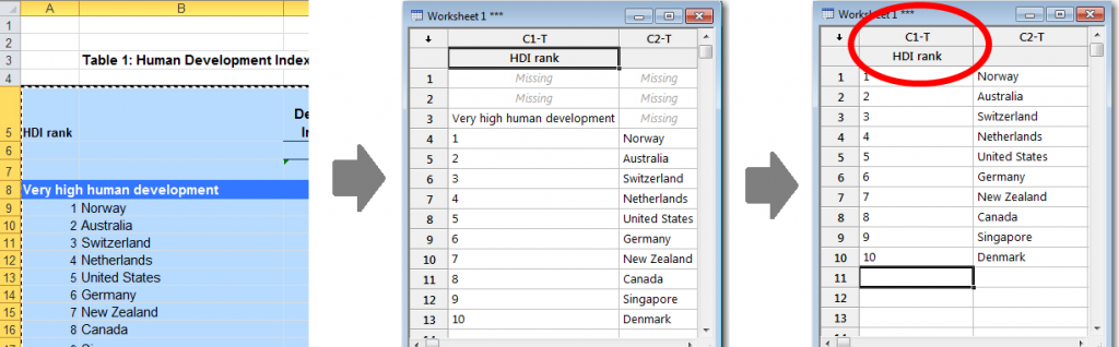
Especially when you copy and paste data, you can find that numeric columns are defined as text. For example, I copied the HDI data from the Excel file that the United Nations Development Programme provides. After pasting the data into Minitab, I deleted the rows at the top that weren't data. Because the first piece of data in the HDI rank column was “Very high human development,” the entire column is still defined as text, even though I wanted the rank to be a number:
In the past, you would have used the Data menu to change the data type. In Minitab 17.2, you can change the data type faster by right-clicking. Here’s how:
- Select a cell in HDI Rank
- Right-click and choose Format Column.
- Select Automatic numeric and click OK.
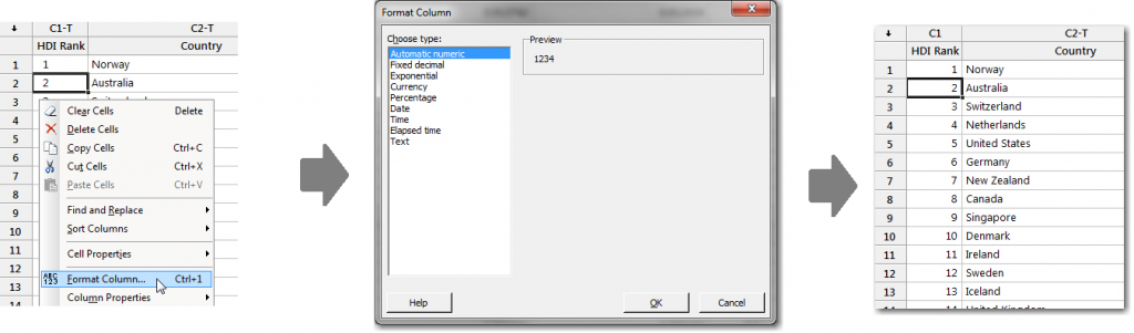
That’s it, you’re done! You can change columns to 9 different formats this way.
Highlighting
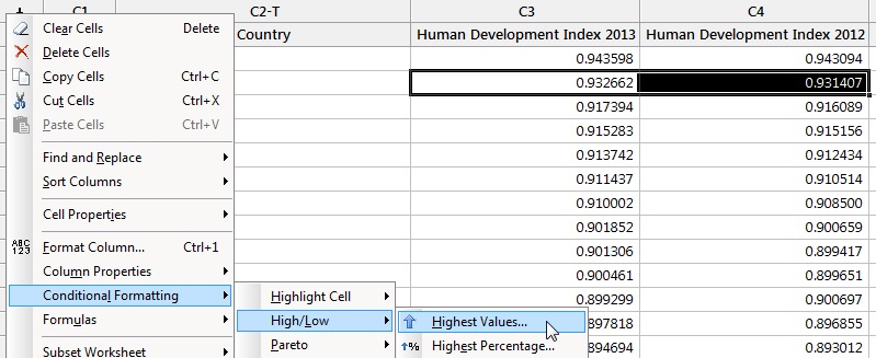
For simple comparisons, it can be just as easy to look at the data in the worksheet as it is to create a graph. Let’s say that you wanted to know if the same 10 countries with the highest HDI Index scores in 2013 had the highest scores in 2012. You can use conditional formatting to quickly highlight the cells of interest to compare two columns:
- Select cells in the columns that you want to format.
- Right-click and choose Conditional Formatting High/Low > Highest Values.
- Click OK.
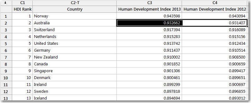
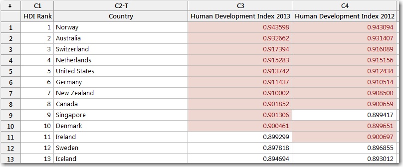
With the conditional formatting, you can quickly see that Singapore moved into the top 10, making Ireland number 11. For another example, see how Cheryl Pammer uses conditional formatting to identify the shortest wait times for rides at Disney World.
Wrap-up
I’ve said it before and I’ll say it again. The only thing better than doing fearless data alanysis is doing fearless data analysis even faster. The new ways that you can use Minitab’s worksheet are meant to help you get the information that you need with as little time and effort as possible. That’s always a good thing.
Bonus
In Minitab’s support center, you can find all sorts of examples about ways that you can conditionally format cells. Check out the list in the Conditional Formatting section in Data and Data Manipulation.