Back when I chose the factors to study for my gummi bear design of experiments, I was thinking about the fact that something like the position of the gummi bear and the position of the fulcrum would probably interact. When I finished collecting the data, I was eager to see if that effect showed up in my analysis.
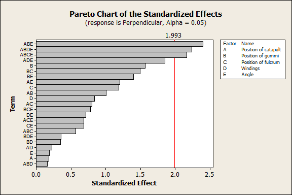
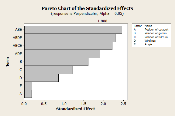
Before we look at the distance parallel to the catapult, let's look at the distance perpendicular to the catapult. I didn’t change any factors with the express purpose of making the gummi bear go left or right, so I was hoping all of these factors would be statistically insignificant. In Minitab, a nice graph to show which DOE effects are significant is a Pareto chart. Here’s the pareto chart when I eliminate effects 1 at a time until all of the effects have p-value below 0.05 or are part of an effect that does.

If I eliminate all the interaction effects with p-values greater than 0.05 one-by one, the same three effects remain significant:

The three significant effects in the perpendicular data are interactions among 3 or more factors:
- Position of catapult, position of gummi, angle
- Position of catapult, position of gummi, number of windings, angle
- Position of catapult, position of gummi, position of fulcrum, angle
Should moving the catapult forward or backward affect how far left or right a gummi bear goes? If it should, should that effect depend on where the gummi bear is on the catapult? And if those two factors depend on each other, should the angle of the gummi bear on the catapult affect the effect of those two? My instinct says “no,” but the data show significance. So what happened? Here are two alternatives to consider in design of experiments.
The effects are statistically significant by chance
Statistical significance allows for the possibility that random variation looks like an effect. The probability that we see an effect by chance is what we control when we choose an alpha value, but be cautious. Alpha is the probability for each hypothesis test individually. The more tests we do, the greater the probability that we see a random effect that is statistically significant.
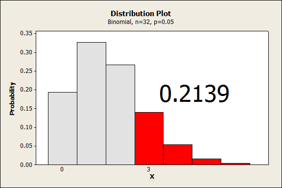
I’ll assume a binomial model is valid for whether an effect is significant or not. This requires assumptions that are not strictly true in this case, but gives an idea of how the probability of making an error increases when we increase the number of tests.
With 32 tests and a probability of 0.05, the probability that we find 3 or more significant effects by chance is 0.2139. That probability is not small enough to ignore, even if it’s not exact.

The effects are from lurking variables
Just because an effect could be random doesn’t mean that the effect is random. The effect could be because of a variable that’s not in the data. I did my best to control all of the factors that could affect how far the gummi bears go parallel to the catapult, but didn’t think as much about the perpendicular direction. For example, while the interactions are hard to understand, it’s easy to see that if the catapult turns, the gummi bear will go further to the left or right. When performing the data collection, I learned that some combinations of the factors make it harder to keep the catapult straight. If the direction of the catapult at launch is confounded with an interaction, we’ll see the effect from the factors even though they’re not the cause. A confounded variable can be a better explanation than a complex interaction.
R2 statistics
We don’t have to look only at statistical significance with models. R2 statistics can tell us about how useful a model is. For example, the R2 statistics for the model of perpendicular distance with all of the terms that are part of the significant terms are these values:
R-Sq = 32.83% R-Sq(pred) = 0.00% R-Sq(adj) = 9.82%For R2 statisics smaller is worse, so these are bad.
The model with the main effects and only the interactions that were significant gives these values:
R-Sq = 20.46% R-Sq(pred) = 0.00% R-Sq(adj) = 11.43%If you spend a lot of time with different models trying to maximize the predicted R2 value, this next model is relatively good, though some terms are not statistically significant.
- Position of gummi
- Position of gummi by position of fulcrum
- Position of gummi by angle
- Position of catapult by position of gummi by angle
- Position of catapult by windings by angle
- Position of catapult by position of gummi by position of fulcrum by angle
- Position of catapult by position of gummi by windings by angle
Seeing these R2 statistics, I feel better. Especially becase R-Sq(pred) tells me about how well this model will predict new values. It looks like whether the effects are real or not, the factors are explaining such a small amount of the variation present that I can still aim my catapult directly at the target. Next time, we’ll explore model-fitting for the parallel distance.
Of course, low p-values aren’t the only ones to think carefully about. If you’re ready for more now, check out Michelle Paret’s thoughts on when a p-value might be misleading!


