


by Matthew Barsalou, guest blogger
We can use a simple catapult to teach process capability analysis using Minitab Statistical Software’s Capability SixpackTM. Here's how.
A process capability analysis is performed to determine if a process is statistically capable. Based on the results of the capability study, we can estimate the amount of defective components the process would produce.
However, a process must be in statistical control and have a normal distribution. A process that is not in statistical control must be brought in control before the capability analysis is performed. In addition, data that does not fit the normal distribution will need to be normalized using a transformation such as the Box-Cox transformation.
The Catapult Setup and First Run
A process and a specification are needed to demonstrate process capability analysis; we used a simple catapult. A rough idea of the catapult’s range and precision was required for determining what the specification should be, so we fired five catapult shots and recorded the distance the projectile traveled. Based on the results, we determined the catapult should be able to consistently land projectiles within a range of one meter. This was just a rough figure used to get started.
We set the specification at 700 cm from the end of a hallway to the point where the projectiles should land. The tolerance was set as +/- 50 cm, which might or might not be a specification that the catapult could meet. The purpose of the study was to determine if the catapult is capable, so the uncertainty was not a problem.
The catapult was then set up 400 cm away from the target of 700 cm.
The First Run and Capability Analysis
The catapult has a rubber band that hooks onto the front of the catapult and then goes over a wire guide that causes additional stretching before the rubber band is mounted onto the catapult arm. The wire guide was replaced with a thin wire that was bent and distorted. Ten shots were fired and the results were recorded. The wire was rotated 22.5° after each shot; rotating a weak and bent wire simulated a cause of variation in the process.
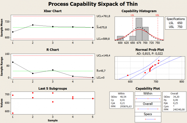
The Minitab Capability Sixpack results for the run using a thin wire are depicted below. Minitab's Capability Sixpack provides a Xbar chart, an R chart, a view of the last five subgroups, a capability histogram, a normal probability plot and a capability plot with capability indices.
The Xbar chart and R chart were automatically calculated by Minitab using the run data that was entered. The specified subgroup size was 2, so each dot in the Xbar chart represents the average of two catapult shots. The average of the averages is 675.8 cm. This is short of the target of 700 cm, but still within specification.
Minitab has calculated the upper control limit (UCL) and lower control limit (LCL). The control limits are 3σ above or below the mean. The UCL is 761.8 cm and the lower control limit is 589.8 cm. The average was within the specification; however, the control limits are +/- 3σ of the process mean and 99.7% of the data will be within the control limits. Unfortunately, the catapult process will result in shots that will be out of specification because the LCL is below the LSL.
Reading the Process Capability Charts
The R chart calculates the average of the ranges in each subgroup of sample size two. The UCL and LCL for the range can be calculated using using the average of the ranges and a table; however, Minitab automatically performs the calculations. Here we can observe a large amount of variation in the catapult results. The actual results of the last five subgroups are also given. The difference between the first and second shot fired was over 100 cm; hence, the large range for the first subgroup in the R chart.
The capability histogram presents a histogram of the results with the shape of the distribution overlaid. The capability histogram also visually depicts the process output compared to the lower specification limit (LSL) and the upper specification limit (USL).
The normal probability plot depicts an Anderson-Darling goodness-of-fit test; this is used to determine if the data follows a normal distribution. The H0 is “data fits the normal distribution” and the Ha is “data does not fit the normal distribution.” The test statistic is automatically calculated by Minitab. Using an alpha of 0.05, we reject the null hypothesis because the calculated P value was only 0.022. This run not only had a large amount of variability; it violated the assumption of normality needed for the calculations.
What's Next in this Capability Analysis?
In my next blog post, I'll perform a second run using thicker and more robust wire to stretch the rubber band. Since this wire will not have the variation that the thin one did, it will simulate a process improvement. We should see a reduction in variability as a result.
In the meantime, if you want to build your own catapult, here are my plans and instructions for the DIY DOE Catapult in a PDF document.