


By Erwin Gijzen, Guest Blogger
In my previous post, we assessed the out-of-spec level for a process with capability analysis and visualized process variability using a control chart. Our goal is to reduce variability, but when a process has a multitude of categorical and continuous variables, identifying root causes can be a huge challenge. Analyzing covariance—using the statistical technique called ANCOVA—can overcome this challenge. In this post, we’ll analyze a real-life data set to learn which variables significantly influenced the final product’s quality.
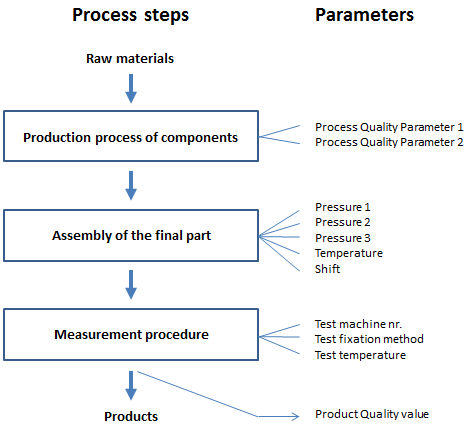
The Process
The Data Set
Our data set contains 874 rows of data collected over a one-month period.
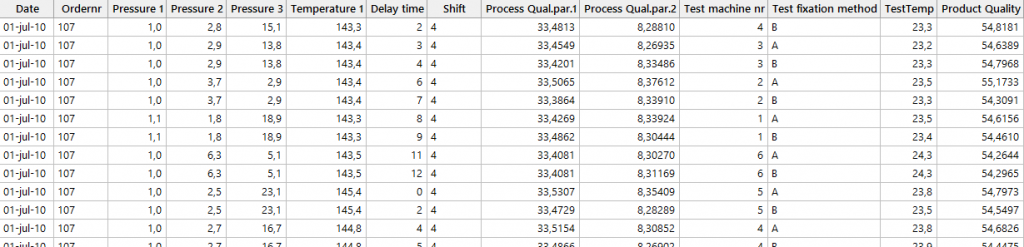
The data include information from several production and measurement steps, as well as the final quality value. The left side of the data sheet, up to and including “Shift,” represents process-related data. The process quality parameters 1 and 2 reflect the quality of previously produced parts. The remaining columns capture data about the test procedure and the final product’s quality.
The Analysis
ANOVA (Analysis of Variance) compares variances among categorical variables. When we include continuous variables—covariates—in the analysis, we can see how much the factors change together. This ANCOVA method uses a general linear model to evaluate the covariates—in this case, pressures, temperatures, delay time, and both process quality parameters—by blending ANOVA with regression analysis.
This analysis is performed in Minitab by selecting Stat > ANOVA > General Linear Model > Fit General Linear Model from the menu, and then selecting the variables. “Factors” are the categorical variables we would use in a traditional ANOVA, while “Covariates” are the continuous data from our process.
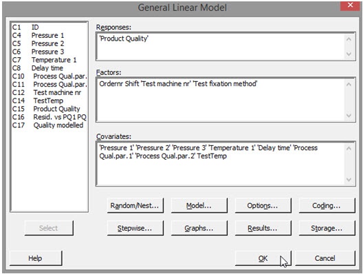
We will want to evaluate the residuals of the analysis for later evaluation. To capture them, simply click “Storage” and then check the “Residuals” box.
The results of the analysis are shown below:
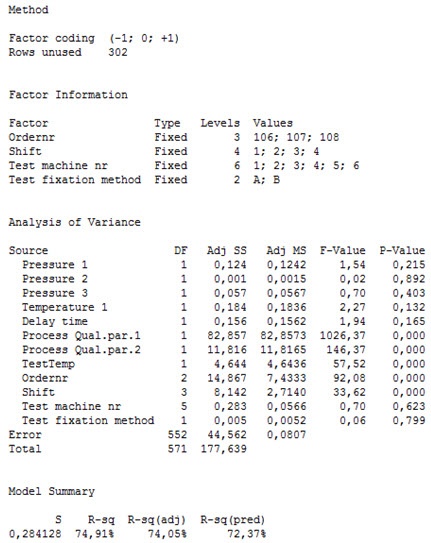
The R-squared is about 75%, which means that about three quarters of the observed variation in our data can be explained by the variables included in the analysis.
When the insignificant terms—those with p-values higher than 0.05—are removed from the analysis, we get the following results:
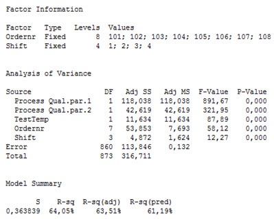
Clearly, with an R2 value of 64%, the model explains a fair piece of the quality variation. The R2 does not need to be very high, as the only intention is to find variables that significantly influence quality.
Using the Residuals to Dig Deeper
Looking at the residuals from this analysis in a control chart gives us additional insight into how controlling the factors in the final model might affect the process:
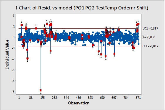
We can use the residuals as an indicator of how the process might behave if the factors in the model were controlled. The red areas let us know where the residuals are still exhibiting unusual variation. They suggest that the variables in the model do not fully cover the causes of the quality variation, so there might be important variables that are not present in the data set. It’s also important to remember that this analysis does not prove a causal relationship between the variables and quality.
To visualize how many out-of-spec products might be produced if we controlled all of the model terms, we can create a new column of data in which we add the mean of our first control chart (shown part 1 of this blog post) to the residuals. Then we create a control chart from that column:
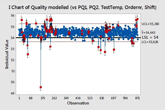
We also can perform a capability analysis on that column of data to see how the process might perform if all terms were fully controlled.
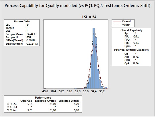
When we compare the graph above to the first process capability graph (from part 1 of this blog post), we see that out-of-spec products would drop from 13.6% to 5.6%, or by 59%.
Managers can now evaluate the benefits of this theoretical drop in quality variation against the engineering resources that would be needed to bring the five significant model terms under control.
Next Steps
The analysis showed that the two process-related quality parameters, test temperature, the order number, and the differences between shifts affect the amount of out-of-spec product. The two process-related quality parameters and the difference between orders account for most of the quality variation since they have the highest “Adj SS” values in the ANCOVA analysis table. This means that the production of the components, before they are assembled into the final product, has a clear influence on the observed quality variation.
ANCOVA analysis provided valuable guidance on eliminating variation from this process, and insight into the resources that might be needed. By comparing the potential benefits of this reduction and to the resources required to fix the causes, decision-makers can make an informed decision about the best course of action.
About the Guest Blogger
Erwin Gijzen, MSc, is a chemical engineer with over 20 years’ experience in process improvement in the chemical, pharmaceutical, and food industries. As owner and senior consultant of Quality Target in the Netherlands, he assists companies in developing products and processes.