A Six Sigma Healthcare Project, part 3: Creating a Binary Logistic Regression Model for Patient Participation

In part 2 of this series, we used graphs and tables to see how individual factors affected rates of patient participation in a cardiac rehabilitation program. This initial look at the data indicated that ease of access to the hospital was a very important contributor to patient participation.

A good estimate of that probability will enable us to calculate the break-even point for such a service. We can use regression to develop a statistical model that lets us do just that.

We have a binary response variable, because only two outcomes exist: a patient either participates in the rehabilitation program, or does not. To model these kinds of responses, we need to use a statistical method called "Binary Logistic Regression." This may sound intimidating, but it's really not as scary as it sounds, especially with a statistical software package like Minitab.

Download the data set to follow along and try these analyses yourself. If you don't already have Minitab, you can download and use our statistical software free for 30 days.

Using Stepwise Binary Logistic Regression to Obtain an Initial Model

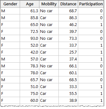
First, let's review our data. We know the gender, age, and distance from the hospital for 500 cardiac patients. We also know whether or not they have access to a vehicle ("Mobility") and whether or not they participated in the rehabilitation program after their surgery (coded so that 0 = no, and 1 = yes). 

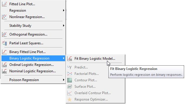
The process of developing a regression equation that can predict a response based on your data is called "Fitting a model." We'll do this in Minitab by selecting Stat > Regression > Binary Logistic Regression > Fit Binary Logistic Model... 

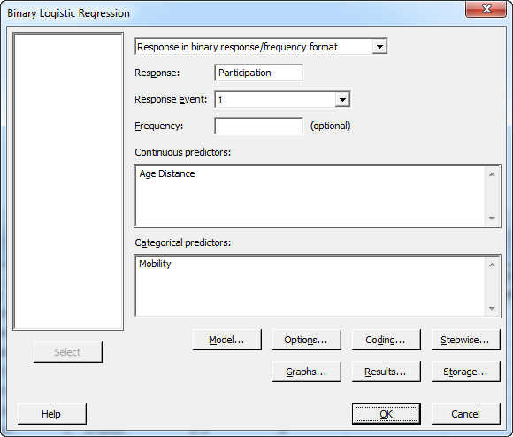
In the dialog box, we need to select the appropriate columns of data for the response we want to predict, and the factors we wish to base the predictions on. In this case, our response variable is "Participation," and we're basing predictions on the continuous factors of "Age" and "Distance," along with the categorical factor "Mobility." 

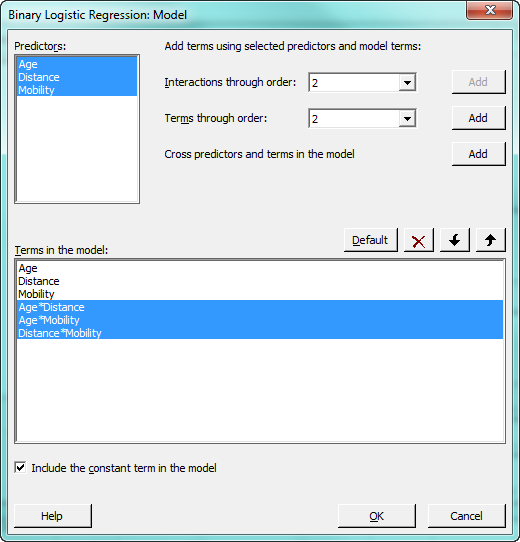
After selecting the factors, click on the "Model" button. This lets us tell Minitab whether we want to consider interactions and polynomial terms in addition to the main effects of each factor. Complete the Model dialog as shown below. To include the two-way interactions in the model, highlight all the items in the Predictors window, make sure that the “Interactions through order:” drop-down reads “2,” and press the Add button next to it:

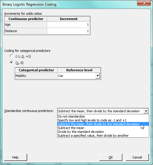
Click OK to return to the main dialog, then press the “Coding” button. In this subdialog, we can tell Minitab to automatically standardize the continuous predictors, Age and Distance. There are several reasons you might want to standardize the continuous predictors, and different ways of standardizing depending on your intent.

In this case, we’re going to standardize by subtracting the mean of the predictor from each row of the predictor column, then dividing the difference by the standard deviation of the predictor. This centers the predictors and also places them on a similar scale. This is helpful when a model contains highly correlated predictors and interaction terms, because standardizing helps reduce multicollinearity and improves the precision of the model’s estimated coefficients. To accomplish this, we just need to select that option from the drop-down as shown below:

After you click OK to return to the main dialog, press the "Stepwise" button. We use this subdialog to perform a stepwise selection, which is a technique that automatically chooses the best model for your data. Minitab will evaluate several different models by adding and removing various factors, and select the one that appears to provide the best fit for the data set. You can have Minitab provide details about the combination of factors it evaluates at each "step," or just show the recommended model.

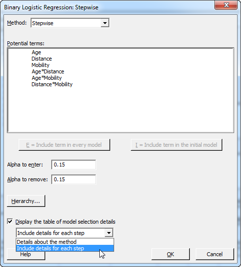
Now click OK to close the Stepwise dialog, and OK again to run the analysis. The output in Minitab's Session window will include details about each potential model, followed by a summary or "deviance" table for the recommended model.

Assessing and Refining the Regression Model

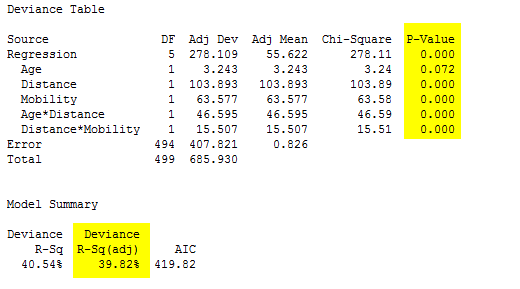
Using software to perform stepwise regression is extremely helpful, but it's always important to check the recommended model to see if it can be refined further. In this case, all of the model terms are significant, and the deviance table's adjusted R² indicates that the model explains about 40 percent of the observed variation in the response data. 

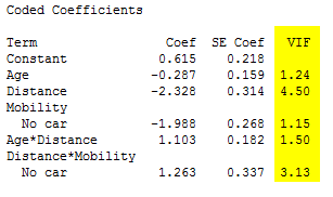
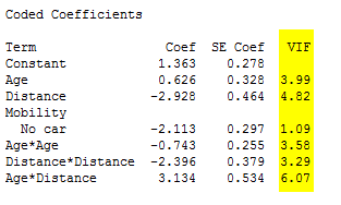
We also want to look at the table of coded coefficients immediately below the summary. The final column of the table lists the VIFs, or variance inflation factors, for each term in the model. This is important because VIF values greater than 5–10 can indicate unstable coefficients that are difficult to interpret.

None of these terms have VIF values over 10.  

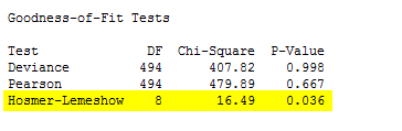
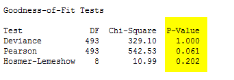
Minitab also performs goodness-of-fit tests that assess how well the model predicts observed data. The first two tests, the deviance and Pearson chi-squared tests, have high p-values, indicating that these tests do not support the conclusion that this model is a poor fit for the data. However, the low p-value for the Hosmer-Lemeshow test indicates that the model could be improved.

It may be that our model does not account for curvature that exists in the data.  We can ask Minitab to add polynomial terms, which model curvature between predictors and the response, to see if it improves the model. Press CTRL-E to recall the binary logistic regression dialog box, then press the "Model" button. To add the polynomial terms, select Age and Distance in the Predictors window, make sure that "2" appears in the “Terms through order:” drop-down, and press "Add" to add those polynomial terms to the model. An order 2 polynomial is the square of the predictor.

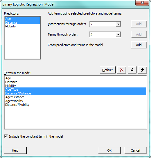
You may have noticed that we did not select “Mobility” above. Why? Because that categorical variable is coded with 1’s and 0’s, so the polynomial term would be identical to the term that is already in the model.

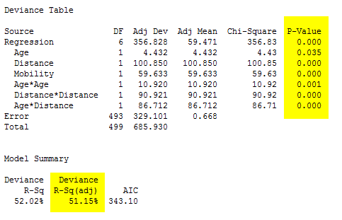
Now press OK all the way out to have Minitab evaluate models that include the polynomial terms. Minitab generates the following output:: 

However, the VIFs for Mobility and the Distance*Mobility interaction remain higher than desirable:

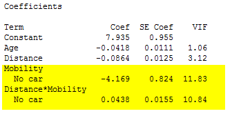
So far, so good—all model terms are significant, and the adjusted R² indicates that the new model accounts for 51 percent of the observed variation in the response, compared to the initial model’s 40 percent. The coefficients are also acceptable, with no variance inflation factors above 10. These terms are moderately correlated, but probably not enough to make the regression results unreliable: 

The goodness-of-fit tests for this model also look good—the lack of p-values below 0.05 indicate that these tests do not suggest the model is a poor fit for the observed data.

The Binary Logistic Regression Equations

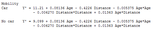
This model seems like the best option for predicting the probability of patient participation in the program. Based on the available data, Minitab has calculated the following regression equations, one that predicts the probability of attendance for people who have access to their own transportation, and one for those who do not:

In the next post, we'll complete this process by using this model to make predictions about the probability of participation in the rehabilitation program and how much we can afford to invest in transportation to help more cardiac patients.