Why the Weibull Distribution Is Always Welcome

In college I had a friend who could go anywhere and fit right in. He'd have lunch with a group of professors, then play hacky-sack with the hippies in the park, and later that evening he'd hang out with the local bikers at the toughest bar in the city. Next day he'd play pickup football with the jocks before going to an all-night LAN party with his gamer pals. On an average weekend he might catch an all-ages show with the small group of straight-edge punk rockers on our campus, or else check out a kegger with some townies, then finish the weekend by playing some D&D with his friends from the physics club.

He was like a chameleon, able to match and reflect the characteristics of the people he was with. That flexibility made him welcome in an astonishingly diverse array of social circles. 

His name was Jeff Weibull, and he was so popular that local statisticians even named "The Weibull Distribution" after him. 

What Makes the Weibull Distribution So Popular? 

All right, I just made that last part up—Jeff's last name wasn't really "Weibull," and the distribution is named for someone else entirely.  But when I first learned about the Weibull Distribution, I immediately recalled Jeff, and his seemingly effortless ability to be perfectly comfortable in such a wide variety of social settings. 

Just as Jeff was a chameleon in different social circles, the Weibull distribution has the ability to assume the characteristics of many different types of distributions. This has made it extremely popular among engineers and quality practitioners, who have made it the most commonly used distribution for modeling reliability data. They like incorporating the Weibull distribution into their data analysis because it is flexible enough to model a variety of data sets. 

Got right-skewed data? Weibull can model that. Left-skewed data? Sure, that's cool with Weibull. Symmetric data? Weibull's up for it. That flexibility is why engineers use the Weibull distribution to evaluate the reliability and material strengths of everything from vacuum tubes and capacitors to ball bearings and relays.

The Weibull distribution can also model hazard functions that are decreasing, increasing or constant, allowing it to describe any phase of an item’s lifetime.

How the Weibull Curve Changes Its Shape

So just how flexible is the Weibull distribution? Let's look at some examples using Graph > Probability Distribution Plot in Minitab Statistical Software. (If you want to follow along and you don't already have Minitab, download the free 30-day trial.) 

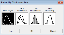
Select "View Single," and then "Weibull" in the Distribution drop-down menu. The dialog box will let you specify three parameters: shape, scale, and threshold.  

The threshold parameter indicates the distribution's shift away from 0, with a negative threshold shifting the distribution to the left of 0, and a positive threshold shifting it to the right. All data must be greater than the threshold. The scale parameter is the 63.2 percentile of the data, and it defines the Weibull curve's relation to the threshold, like the mean defines a normal curve's position. For our examples we'll use a scale of 10, which says that 63.2% of the items tested will fail in the first 10 hours following the threshold time. The shape parameter, describes the shape of the Weibull curve. By changing the shape, you can model the characteristics of many different life distributions.

For this post, I'll focus exclusively on how the shape parameter affects the Weibull curve. I'll go through these one-by-one, but if you'd like to see them all together on a single plot, choose the "Vary Parameters" option in the dialog box shown above. 

Weibull Distribution with Shape Less Than 1

Let's start with a shape between 0 and 1. The graph below shows the probability decreases exponentially from infinity. In terms of failure rate, data that fit this distribution have a high number of initial failures, which decrease over time as the defective items are eliminated from the sample. These early failures are frequently called "infant mortality," because they occur in the early stage of a product's life.  

Weibull Distribution with Shape Equal to 1

When the shape is equal to 1, the Weibull distribution decreases exponentially from 1/alpha, where alpha = the scale parameter. Essentially, this means that over time the failure rate remains consistent. This shape of the Weibull distribution is appropriate for random failures and multiple-cause failures, and can be used to model the useful life of products. 

Weibull Distribution with Shape Between 1 and 2

When the shape value is between 1 and 2, the Weibull Distribution rises to a peak quickly, then decreases over time. The failure rate increases overall, with the most rapid increase occurring initially. This shape is indicative of early wear-out failures. 

Weibull Distribution with Shape Equal to 2

When the shape value reaches 2, the Weibull distribution models a linearly increasing failure rate, where the risk of wear-out failure increases steadily over the product's lifetime. This form of the Weibull distribution is also known as the Rayleigh distribution. 

Weibull Distribution with Shape Between 3 and 4

If we put the shape value between 3 and 4, the Weibull distribution becomes symmetric and bell-shaped, like the normal curve. This form of the Weibull distribution models rapid wear-out failures during the final period of product life, when most failures happen.

Weibull Distribution with Shape Greater than 10

When the shape value is above 10, the Weibull distribution is similar to an extreme value distribution. Again, this form of the distribution can model the final period of product life. 

Is Weibull Always the Best Choice? 

When it comes to reliability, Weibull frequently is the go-to distribution, but it's important to note other distribution families can model a variety of distributional shapes, too. You want to find the distribution that gives you the best fit for your data, and that may not be a form of the Weibull distribution. For example, product failures caused by chemical reactions or corrosion are usually modeled with the lognormal distribution.

You can assess the fit of your data using Minitab’s Distribution ID plot (Stat > Reliability/Survival > Distribution Analysis (Right-Censoring or Arbitrary Censoring)). If you want more details about that, check out this post Jim Frost wrote about identifying the distribution of your data.  

Case study:
Time-to-Market and Design for Reliability at the Speed of Light in Signify

Get ready for a light bulb moment! In a fast-changing industry where time-to-market and product reliability give a competitive edge, discover how the world’s leading lighting company Signify, rapidly validates new innovations. In this one hour webinar, Prof W.D. van Driel and Dr P. Watté will shed a light on design for reliability (DfR) using Minitab Statistical Software at Signify, the former Philips Lighting. Learn from real-life examples their methods to lower your development costs, improve your designs’ performance and compliance, and accelerate the testing of product design reliability. If you develop products intended to meet high specifications for years to come, you will discover how to reduce the risks and consequences of product failure and costly claims - for you and your customers.