Curing Heteroscedasticity with Weighted Regression in Minitab Statistical Software

In my last post I talked about why you need to check your regression analysis residuals. In a nutshell, your predictors should be so good at explaining (or predicting) the response that only the inherent randomness of any real-world phenomenon remains leftover for the error portion. If you observe explanatory or predictive power in the error, you know that your predictors are missing some of the predictive information. In this post I'll cover a specific type of pattern that you can see in the residuals and show you how to fix the problem.

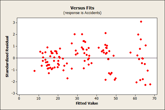
Regression residuals should have a constant spread across all fitted values. If your plot looks like the one below, you've got a problem known as heteroscedasticity or non-constant variance. You can see that as the fitted values get larger, so does the vertical spread of the residuals. That increasing spread represents predictive information that is leaking over into your residual plot. If you can figure out why the variability of your residuals change, you can improve your analyses accordingly.

Why fix the problem? There are two big reasons:

• The precision of the coefficient estimates is lower with non-constant variance.
• The p-values for the regression coefficients are based on satisfying the assumption of constant variance. Therefore, your p-values, and the associated decisions about the statistical significance of your predictors, can be incorrect if your residuals have non-constant variance.

Today, I'll look at a common solution that Minitab statistical software provides, weighted regression.

Case Study: Accidents by Population

We'll model the number of car accidents as a function of the population. You can download the data to do this yourself. This is not real-world data but it accurately reflects the problem and the cure.

1. Open the worksheet and go to Stat > Regression > Regression > Fit Regression Model.
2. In Responses, enter Accidents.
3. In Continuous predictors, enter Population.
4. Click Graphs.
5. Choose Standardized* and then check Residuals versus fits.
6. Click OK in all dialog boxes.

*It is crucial to use standardized residuals. Regular residuals will show us the problem with non-constant variance. However, only standardized residuals will show us that we have fixed the problem. Standardized residuals have other benefits as well, but that's the subject of another post.

After running the analysis, out pops the Residual versus fits graph that is shown above. As we assess the model, we notice that this graph displays residuals with non-constant variance. For this example, we'll only look at the Residuals versus fits plots that we create because it is the only place where we can see the heteroscedasticity.

Cross-sectional studies, such as this one, are at a greater risk of exhibiting heteroskedasticity due to a greater disparity between the largest and smallest values of a predictor. Think of small towns versus the large cities! In this case, we focus on population size because the values vary greatly. It is likely that the variance of the error increases with the size of the population.

Using Weighted Regression

Weighted regression is one method that you can use to correct the residuals. Determining the proper weight to use can be a challenging task and requires subject-area knowledge. This procedure is particularly useful when you can identify a variable that changes with the variance of the residuals.

For the reasons discussed above, the weights in this example are based on the population variable. I created a column of weights by calculating the reciprocal of the population (1/population) for each row. You can do this in Minitab with the tools in Calc > Calculator.

Weighted regression works by weighting each data point based on the variability of it's fitted value. In this case, data points with a larger population have residuals with a higher variance. We want to give places with a higher population a lower weight in order to shrink their squared residuals. With the proper weight, this procedure minimizes the sum of weighted squared residuals to produce residuals with a constant variance (homoskedasticity).

So, let's rerun this analysis with the column of weights.

1. Go to Stat > Regression > Regression > Fit Regression Model.
2. In Responses, enter Accidents.
3. In Continuous predictors, enter Population.
4. Click Options.
5. In Weights, enter Weight.
6. Click Graphs.
7. Choose Standardized and then check Residuals versus fits.
8. Click OK in all dialog boxes.

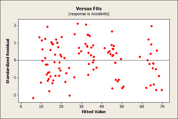
Out pops another Residuals versus fits plot!

This one looks much better! The vertical spread of the residuals is consistent across the range of fitted values. We've cured the case of heteroscedasticity!

Closing Thoughts

We've just compared the residual plots and it is clear that weighted regression produced better residuals than the regular regression. We can trust the weighted regression results.

If you like, you can compare the output in the session window. However, the differences between any given pair of weighted and unweighted analyses is unpredictable. The general takeaway here is that in this type of situation you can trust the weighted results more than the unweighted results.

Keep in mind that there are different reasons why residuals can have non-constant variance. We tackled one that involved a predictor variable that had a large range of values and was associated with the changing variance. Other reasons for heteroscedasticity can include an incorrect model, such as a missing predictor. Weighted regression is not an appropriate solution if the heteroskedasticity is caused by an omitted variable. So, you really have to use your subject-area knowledge to first determine what is causing the problem and then figure out how to fix it!