


Data mining uses algorithms to explore correlations in data sets. An automated procedure sorts through large numbers of variables and includes them in the model based on statistical significance alone. No thought is given to whether the variables and the signs and magnitudes of their coefficients make theoretical sense.
We tend to think of data mining in the context of big data, with its huge databases and servers stuffed with information. However, it can also occur on the smaller scale of a research study.
The comment below is a real one that illustrates this point.
“Then, I moved to the Regression menu and there I could add all the terms I wanted and more. Just for fun, I added many terms and performed backward elimination. Surprisingly, some terms appeared significant and my R-squared Predicted shot up. To me, your concerns are all taken care of with R-squared Predicted. If the model can still predict without the data point, then that's good.”
Comments like this are common and emphasize the temptation to select regression models by trying as many different combinations of variables as possible and seeing which model produces the best-looking statistics. The overall gist of this type of comment is, "What could possibly be wrong with using data mining to build a regression model if the end results are that all the p-values are significant and the various types of R-squared values are all high?"
In this blog post, I’ll illustrate the problems associated with using data mining to build a regression model in the context of a smaller-scale analysis.
An Example of Using Data Mining to Build a Regression Model
My first order of business is to prove to you that data mining can have severe problems. I really want to bring the problems to life so you'll be leery of using this approach. Fortunately, this is simple to accomplish because I can use data mining to make it appear that a set of randomly generated predictor variables explains most of the changes in a randomly generated response variable!
To do this, I’ll create a worksheet in Minitab statistical software that has 100 columns, each of which contains 30 rows of entirely random data. In Minitab, you can use Calc > Random Data > Normal to create your own worksheet with random data, or you can use this worksheet that I created for the data mining example below. (If you don’t have Minitab and want to try this out, get the free 30 day trial!)
Next, I’ll perform stepwise regression using column 1 as the response variable and the other 99 columns as the potential predictor variables. This scenario produces a situation where stepwise regression is forced to dredge through 99 variables to see what sticks, which is a key characteristic of data mining.
When I perform stepwise regression, the procedure adds 28 variables that explain 100% of the variance! Because we only have 30 observations, we’re clearly overfitting the model. Overfitting the model is different problem that also inflates R-squared, which you can read about in my post about the dangers of overfitting models.
I’m specifically addressing the problems of data mining in this post, so I don’t want a model that is also overfit. To avoid an overfit model, a good rule of thumb is to include no more than one term for each 10 observations. We have 30 observations, so I’ll include only the first three variables that the stepwise procedure adds to the model: C7, C77, and C95. The output for the first three steps is below.
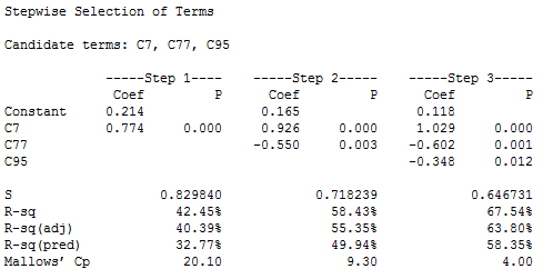
Under step 3, we can see that all of the coefficient p-values are statistically significant. The R-squared value of 67.54% can either be good or mediocre depending on your field of study. In a real study, there are likely to be some real effects mixed in that would boost the R-squared even higher. We can also look at the adjusted and predicted R-squared values and neither one suggests a problem.
If we look at the model building process of steps 1 - 3, we see that at each step all of the R-squared values increase. That’s what we like to see. For good measure, let’s graph the relationship between the predictor (C7) and the response (C1). After all, seeing is believing, right?
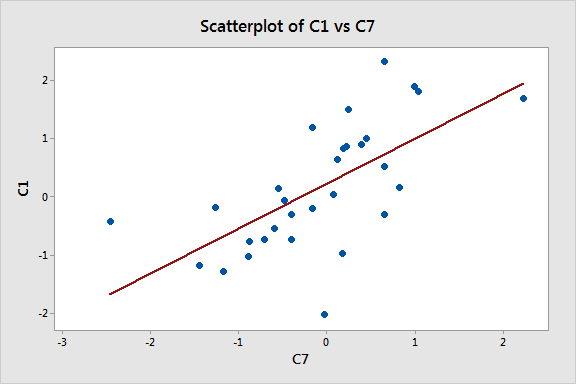
This graph looks good too! It sure appears that as C7 increases, C1 tends to increase, which agrees with the positive regression coefficient in the output. If we didn’t know better, we’d think that we have a good model!
This example answers the question posed at the beginning: what could possibly be wrong with this approach? Data mining can produce deceptive results. The statistics and graph all look good but these results are based on entirely random data with absolutely no real effects. Our regression model suggests that random data explain other random data even though that's impossible. Everything looks great but we have a lousy model.
The problems associated with using data mining are real, but how the heck do they happen? And, how do you avoid them? Read my next post to learn the answers to these questions!