In this series of posts, I show how hypothesis tests and confidence intervals work by focusing on concepts and graphs rather than equations and numbers.
Previously, I used graphs to show what statistical significance really means. In this post, I’ll explain both confidence intervals and confidence levels, and how they’re closely related to P values and significance levels.
How to Correctly Interpret Confidence Intervals and Confidence Levels
A confidence interval is a range of values that is likely to contain an unknown population parameter. If you draw a random sample many times, a certain percentage of the confidence intervals will contain the population mean. This percentage is the confidence level.
Most frequently, you’ll use confidence intervals to bound the mean or standard deviation, but you can also obtain them for regression coefficients, proportions, rates of occurrence (Poisson), and for the differences between populations.
Just as there is a common misconception of how to interpret P values, there’s a common misconception of how to interpret confidence intervals. In this case, the confidence level is not the probability that a specific confidence interval contains the population parameter.
The confidence level represents the theoretical ability of the analysis to produce accurate intervals if you are able to assess many intervals and you know the value of the population parameter. For a specific confidence interval from one study, the interval either contains the population value or it does not—there’s no room for probabilities other than 0 or 1. And you can't choose between these two possibilities because you don’t know the value of the population parameter.
"The parameter is an unknown constant and no probability statement concerning its value may be made."
—Jerzy Neyman, original developer of confidence intervals.
This will be easier to understand after we discuss the graph below . . .
With this in mind, how do you interpret confidence intervals?
Confidence intervals serve as good estimates of the population parameter because the procedure tends to produce intervals that contain the parameter. Confidence intervals are comprised of the point estimate (the most likely value) and a margin of error around that point estimate. The margin of error indicates the amount of uncertainty that surrounds the sample estimate of the population parameter.
In this vein, you can use confidence intervals to assess the precision of the sample estimate. For a specific variable, a narrower confidence interval [90 110] suggests a more precise estimate of the population parameter than a wider confidence interval [50 150].
Confidence Intervals and the Margin of Error
Let’s move on to see how confidence intervals account for that margin of error. To do this, we’ll use the same tools that we’ve been using to understand hypothesis tests. I’ll create a sampling distribution using probability distribution plots, the t-distribution, and the variability in our data. We'll base our confidence interval on the energy cost data set that we've been using.
When we looked at significance levels, the graphs displayed a sampling distribution centered on the null hypothesis value, and the outer 5% of the distribution was shaded. For confidence intervals, we need to shift the sampling distribution so that it is centered on the sample mean and shade the middle 95%.
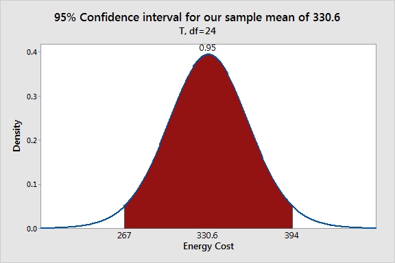
The shaded area shows the range of sample means that you’d obtain 95% of the time using our sample mean as the point estimate of the population mean. This range [267 394] is our 95% confidence interval.
Using the graph, it’s easier to understand how a specific confidence interval represents the margin of error, or the amount of uncertainty, around the point estimate. The sample mean is the most likely value for the population mean given the information that we have. However, the graph shows it would not be unusual at all for other random samples drawn from the same population to obtain different sample means within the shaded area. These other likely sample means all suggest different values for the population mean. Hence, the interval represents the inherent uncertainty that comes with using sample data.
You can use these graphs to calculate probabilities for specific values. However, notice that you can’t place the population mean on the graph because that value is unknown. Consequently, you can’t calculate probabilities for the population mean, just as Neyman said!
Why P Values and Confidence Intervals Always Agree About Statistical Significance
You can use either P values or confidence intervals to determine whether your results are statistically significant. If a hypothesis test produces both, these results will agree.
The confidence level is equivalent to 1 – the alpha level. So, if your significance level is 0.05, the corresponding confidence level is 95%.
- If the P value is less than your significance (alpha) level, the hypothesis test is statistically significant.
- If the confidence interval does not contain the null hypothesis value, the results are statistically significant.
- If the P value is less than alpha, the confidence interval will not contain the null hypothesis value.
For our example, the P value (0.031) is less than the significance level (0.05), which indicates that our results are statistically significant. Similarly, our 95% confidence interval [267 394] does not include the null hypothesis mean of 260 and we draw the same conclusion.
To understand why the results always agree, let’s recall how both the significance level and confidence level work.
- The significance level defines the distance the sample mean must be from the null hypothesis to be considered statistically significant.
- The confidence level defines the distance for how close the confidence limits are to sample mean.
Both the significance level and the confidence level define a distance from a limit to a mean. Guess what? The distances in both cases are exactly the same!
The distance equals the critical t-value * standard error of the mean. For our energy cost example data, the distance works out to be $63.57.
Imagine this discussion between the null hypothesis mean and the sample mean:
Null hypothesis mean, hypothesis test representative: Hey buddy! I’ve found that you’re statistically significant because you’re more than $63.57 away from me!
Sample mean, confidence interval representative: Actually, I’m significant because you’re more than $63.57 away from me!
Very agreeable aren’t they? And, they always will agree as long as you compare the correct pairs of P values and confidence intervals. If you compare the incorrect pair, you can get conflicting results, as shown by common mistake #1 in this post.
Closing Thoughts
In statistical analyses, there tends to be a greater focus on P values and simply detecting a significant effect or difference. However, a statistically significant effect is not necessarily meaningful in the real world. For instance, the effect might be too small to be of any practical value.
It’s important to pay attention to the both the magnitude and the precision of the estimated effect. That’s why I'm rather fond of confidence intervals. They allow you to assess these important characteristics along with the statistical significance. You'd like to see a narrow confidence interval where the entire range represents an effect that is meaningful in the real world.
If you like this post, you might want to read the previous posts in this series that use the same graphical framework:
- Part One: Why We Need to Use Hypothesis Tests
- Part Two: Significance Levels (alpha) and P values
For more about confidence intervals, read my post where I compare them to tolerance intervals and prediction intervals.
If you'd like to see how I made the probability distribution plot, please read: How to Create a Graphical Version of the 1-sample t-Test.