T-tests are handy hypothesis tests in statistics when you want to compare means. You can compare a sample mean to a hypothesized or target value using a one-sample t-test. You can compare the means of two groups with a two-sample t-test. If you have two groups with paired observations (e.g., before and after measurements), use the paired t-test.
How do t-tests work? How do t-values fit in? In this series of posts, I’ll answer these questions by focusing on concepts and graphs rather than equations and numbers. After all, a key reason to use statistical software like Minitab is so you don’t get bogged down in the calculations and can instead focus on understanding your results.
In this post, I will explain t-values, t-distributions, and how t-tests use them to calculate probabilities and assess hypotheses.
What Are t-Values?
T-tests are called t-tests because the test results are all based on t-values. T-values are an example of what statisticians call test statistics. A test statistic is a standardized value that is calculated from sample data during a hypothesis test. The procedure that calculates the test statistic compares your data to what is expected under the null hypothesis.
Each type of t-test uses a specific procedure to boil all of your sample data down to one value, the t-value. The calculations behind t-values compare your sample mean(s) to the null hypothesis and incorporates both the sample size and the variability in the data. A t-value of 0 indicates that the sample results exactly equal the null hypothesis. As the difference between the sample data and the null hypothesis increases, the absolute value of the t-value increases.
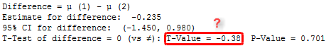
Assume that we perform a t-test and it calculates a t-value of 2 for our sample data. What does that even mean? I might as well have told you that our data equal 2 fizbins! We don’t know if that’s common or rare when the null hypothesis is true.
By itself, a t-value of 2 doesn’t really tell us anything. T-values are not in the units of the original data, or anything else we’d be familiar with. We need a larger context in which we can place individual t-values before we can interpret them. This is where t-distributions come in.
What Are t-Distributions?
When you perform a t-test for a single study, you obtain a single t-value. However, if we drew multiple random samples of the same size from the same population and performed the same t-test, we would obtain many t-values and we could plot a distribution of all of them. This type of distribution is known as a sampling distribution.
Fortunately, the properties of t-distributions are well understood in statistics, so we can plot them without having to collect many samples! A specific t-distribution is defined by its degrees of freedom (DF), a value closely related to sample size. Therefore, different t-distributions exist for every sample size. You can graph t-distributions using Minitab’s probability distribution plots.
T-distributions assume that you draw repeated random samples from a population where the null hypothesis is true. You place the t-value from your study in the t-distribution to determine how consistent your results are with the null hypothesis.
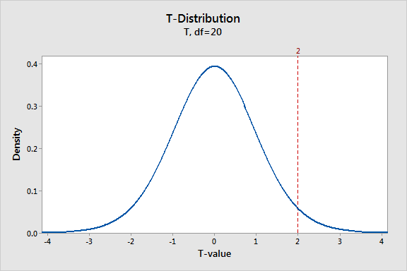
The graph above shows a t-distribution that has 20 degrees of freedom, which corresponds to a sample size of 21 in a one-sample t-test. It is a symmetric, bell-shaped distribution that is similar to the normal distribution, but with thicker tails. This graph plots the probability density function (PDF), which describes the likelihood of each t-value.
The peak of the graph is right at zero, which indicates that obtaining a sample value close to the null hypothesis is the most likely. That makes sense because t-distributions assume that the null hypothesis is true. T-values become less likely as you get further away from zero in either direction. In other words, when the null hypothesis is true, you are less likely to obtain a sample that is very different from the null hypothesis.
Our t-value of 2 indicates a positive difference between our sample data and the null hypothesis. The graph shows that there is a reasonable probability of obtaining a t-value from -2 to +2 when the null hypothesis is true. Our t-value of 2 is an unusual value, but we don’t know exactly how unusual. Our ultimate goal is to determine whether our t-value is unusual enough to warrant rejecting the null hypothesis. To do that, we'll need to calculate the probability.
Ready for a demo of Minitab Statistical Software? Just ask!

Using t-Values and t-Distributions to Calculate Probabilities
The foundation behind any hypothesis test is being able to take the test statistic from a specific sample and place it within the context of a known probability distribution. For t-tests, if you take a t-value and place it in the context of the correct t-distribution, you can calculate the probabilities associated with that t-value.
A probability allows us to determine how common or rare our t-value is under the assumption that the null hypothesis is true. If the probability is low enough, we can conclude that the effect observed in our sample is inconsistent with the null hypothesis. The evidence in the sample data is strong enough to reject the null hypothesis for the entire population.
Before we calculate the probability associated with our t-value of 2, there are two important details to address.
First, we’ll actually use the t-values of +2 and -2 because we’ll perform a two-tailed test. A two-tailed test is one that can test for differences in both directions. For example, a two-tailed 2-sample t-test can determine whether the difference between group 1 and group 2 is statistically significant in either the positive or negative direction. A one-tailed test can only assess one of those directions.
Second, we can only calculate a non-zero probability for a range of t-values. As you’ll see in the graph below, a range of t-values corresponds to a proportion of the total area under the distribution curve, which is the probability. The probability for any specific point value is zero because it does not produce an area under the curve.
With these points in mind, we’ll shade the area of the curve that has t-values greater than 2 and t-values less than -2.
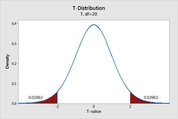
The graph displays the probability for observing a difference from the null hypothesis that is at least as extreme as the difference present in our sample data while assuming that the null hypothesis is actually true. Each of the shaded regions has a probability of 0.02963, which sums to a total probability of 0.05926. When the null hypothesis is true, the t-value falls within these regions nearly 6% of the time.
This probability has a name that you might have heard of—it’s called the p-value! While the probability of our t-value falling within these regions is fairly low, it’s not low enough to reject the null hypothesis using the common significance level of 0.05.
Learn how to correctly interpret the p-value.
t-Distributions and Sample Size
As mentioned above, t-distributions are defined by the DF, which are closely associated with sample size. As the DF increases, the probability density in the tails decreases and the distribution becomes more tightly clustered around the central value. The graph below depicts t-distributions with 5 and 30 degrees of freedom.
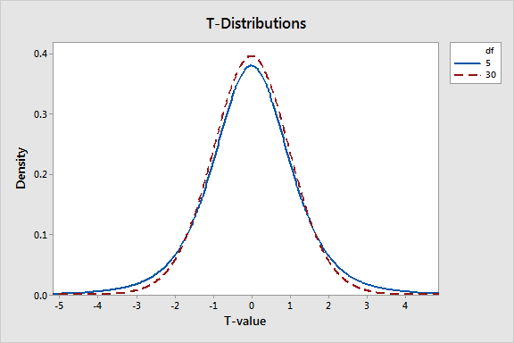
The t-distribution with fewer degrees of freedom has thicker tails. This occurs because the t-distribution is designed to reflect the added uncertainty associated with analyzing small samples. In other words, if you have a small sample, the probability that the sample statistic will be further away from the null hypothesis is greater even when the null hypothesis is true.
Small samples are more likely to be unusual. This affects the probability associated with any given t-value. For 5 and 30 degrees of freedom, a t-value of 2 in a two-tailed test has p-values of 10.2% and 5.4%, respectively. Large samples are better!
I’ve showed how t-values and t-distributions work together to produce probabilities. To see how each type of t-test works and actually calculates the t-values, read the other post in this series, Understanding t-Tests: 1-sample, 2-sample, and Paired t-Tests.
If you'd like to learn how the ANOVA F-test works, read my post, Understanding Analysis of Variance (ANOVA) and the F-test.