


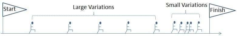
Imagine that you are watching a race and that you are located close to the finish line. When the first and fastest runners complete the race, the differences in times between them will probably be quite small.
Now wait until the last runners arrive and consider their finishing times. For these slowest runners, the differences in completion times will be extremely large. This is due to the fact that for longer racing times a small difference in speed will have a significant impact on completion times, whereas for the fastest runners, small differences in speed will have a small (but decisive) impact on arrival times.
This phenomenon is called “heteroscedasticity” (non-constant variance). In this example, the amount of Variation depends on the average value (small variations for shorter completion times, large variations for longer times).
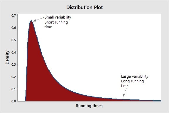
This distribution of running times data will probably not follow the familiar bell-shaped curve (a.k.a. the normal distribution). The resulting distribution will be asymmetrical with a longer tail on the right side. This is because there's small variability on the left side with a short tail for smaller running times, and larger variability for longer running times on the right side, hence the longer tail.
Why does this matter?
- Model bias and spurious interactions: If you are performing a regression or a design of experiments (any statistical modelling), this asymmetrical behavior may lead to a bias in the model. If a factor has a significant effect on the average speed, because the variability is much larger for a larger average running time, many factors will seem to have a stronger effect when the mean is larger. This is not due, however, to a true factor effect but rather to an increased amount of variability that affects all factor effect estimates when the mean gets larger. This will probably generate spurious interactions due to a non-constant variation, resulting in a very complex model with many (spurious and unrealistic) interactions.
- If you are performing a standard capability analysis, this analysis is based on the normality assumption. A substantial departure from normality will bias your capability estimates.
The Box-Cox Transformation
One solution to this is to transform your data into normality using a Box-Cox transformation. Minitab will select the best mathematical function for this data transformation. The objective is to obtain a normal distribution of the transformed data (after transformation) and a constant variance.
Consider the asymmetrical function below :
![]()
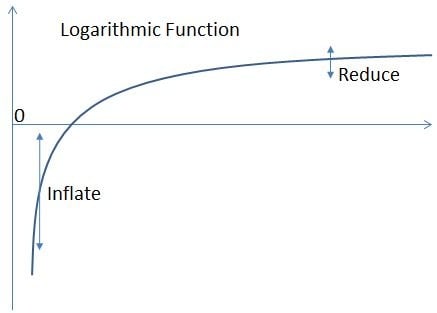
If a logarithmic transformation is applied to this distribution, the differences between smaller values will be expanded (because the slope of the logarithmic function is steeper when values are small) whereas the differences between larger values will be reduced (because of the very moderate slope of the log distribution for larger values). If you inflate differences on the left tail and reduce differences on the right side tail, the result will be a symmetrical normal distribution, and a variance that is now constant (whatever the mean). This is the reason why in the Minitab Assistant, a Box- Cox transformation is suggested whenever this is possible for non-normal data, and why in the Minitab regression or DOE (design of experiments) dialogue boxes, the Box-Cox transformation is an option that anyone may consider if needed to transform residual data into normality.
![]()
The diagram above illustrates how, thanks to a Box-Cox transformation, performed by the Minitab Assistant (in a capability analysis), an asymmetrical distribution has been transformed into a normal symmetrical distribution (with a successful normality test).
Box-Cox Transformation and Variable Scale
Note that Minitab will search for the best transformation function, which may not necessarily be a logarithmic transformation.
As a result of this transformation, the physical scale of your variable may be altered. When looking at a capability graph, one may not recognize his typical values for the variable scale (after transformation). However, the estimated Ppk and Pp capability indices will be reliable and based on a normal distribution. Similarly, in a regression model, you need to be aware that the coefficients will be modified, although the transformation is obviously useful to remove spurious interactions and to identify the factors that are really significant.