Here at Minitab we have a quite a few coffee drinkers. From personal observation, it seemed as if people who are more outgoing are the ones doing most of the coffee drinking, while people who are less outgoing seem to opt for tea. I’d noticed this over a period of time, and eventually decided to investigate.
To test out my hypothesis, I decided to pester some of my coworkers by asking them to participate in my beverage choice survey. Given that the data I collected is categorical rather than continuous, this also seemed like a great way to showcase some of Minitab’s tools for analyzing categorical data.
I surveyed 50 individuals, asking each just two questions: 1) Do you prefer coffee or tea, and 2) Do you consider yourself an introvert or an extrovert? The raw data was entered in a Minitab worksheet as two separate columns. Just for fun, I also generated some pie charts to help me visualize the data.
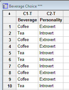
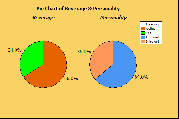
The next thing I did was to summarize the data using Descriptive Statistics (Stat > Tables > Descriptive Statistics):
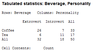
Already, it looks like I may be on to something! We can see from the summarized data that extroverts appear to prefer coffee. But how can we assess if a relationship exists between beverage choice and personality type? Is there a statistically significant relationship here? To answer this question, we can use a Chi-Square test.
What Is a Chi-Square Test?
A Chi-Square test of association does just what the name implies: it tests to see if there is an association between categorical variables. The null hypothesis for the test is that no association exists between the variables. Since my data is in raw format, I used the Cross Tabulation and Chi-Square option in Minitab. The results of the test are shown below:
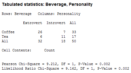
Minitab displays two chi-square statistics: The Pearson Chi-Square statistic is 9.212, and its corresponding p-value is quite low at 0.002. The other Chi-Square statistic we have is the Likelihood-Ratio Chi-Square which has a value of 9.162 and also has a low p-value of 0.002.
Given this information, we reject the null hypothesis of no association and conclude that there is in fact a relationship between personality and beverage choice.
Odds Ratio
What else can we learn from this data? We can easily calculate the odds ratio for this 2x2 table. An odds ratio compares the odds of two events, where the odds of an event equals the probability the event occurs divided by the probability that it does not occur. For our example, the ‘event’ is preferring coffee. For the data in the table above, the calculation is (26*11)/(6*7) = 6.8. An odds ratio of 6.8 tells us that Extroverts are more than six times as likely to choose coffee over tea compared with introverts.
Logistic Regression
Another way to look at this data is to use a logistic regression. A logistic regression models a relationship between predictor variables and a categorical response variable. In Minitab, you can choose from three types of logistic regression (binary, nominal or ordinal), depending on the nature of your categorical response variable. For our example, we will use binary logistic regression because the response variable has two levels (the response being the beverage choice of coffee or tea).
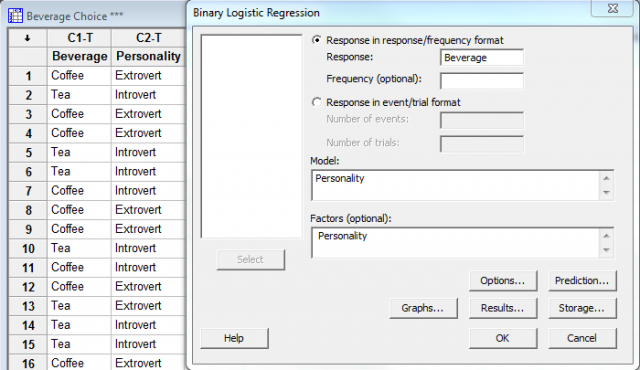
The binary logistic regression option in Minitab is available under Stat > Regression > Binary Logistic Regression. Because my only predictor (Personality) is categorical, I must enter it in the Model field as well as the Factor field in the dialog box:
To understand the output, we need to know the reference event for the response. Minitab needs to designate one of the response values (Coffee or Tea) as the reference event. The default setting for text factors is that the reference event is the last in alphabetical order (so by default it would be Tea). Since I’m really interested in knowing who prefers coffee, I can change the reference event to Coffee by clicking the Options button in the binary logistic regression dialog box and making the change in the Event field:
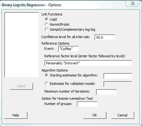
In Minitab, we can also specify the factor level reference (Introvert or Extrovert). The estimated coefficients are then interpreted relative to this reference level. For text factors, the reference level is the level that is first in alphabetical order by default (so Extrovert would be the default). I want the reference level to be Introvert instead so I also made that change in the above dialog box.
Clicking OK in each dialog box gave me the results below:
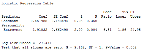
The negative coefficient for the Constant (-0.451985) is the effect on the beverage choice for introverts, and they are less likely to choose coffee than extroverts. The positive coefficient for Extrovert indicates that extroverts are more likely than introverts to choose coffee over tea.
The p-value for Extrovert (0.004) indicates that Personality is a significant predictor of Beverage Choice. Additionally, since we have only one predictor, the odds ratio (6.81) is consistent with the odds ratio that was estimated from the 2x2 table.
As a final step, I used one of the count data macros from Minitab’s macros library to generate an ROC curve, which summarizes the predictive power of this model:
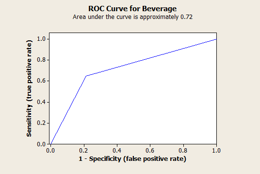
For the ROC curve, the better the predictive power, the higher the curve. An area under the curve of 1 represents a perfect test, and an area of 0.5 (a straight diagonal line from the lower left corner to the upper right corner) represents a pretty worthless model. For this model, the area under the curve = 0.72, so the predictive power of the model is fair.
I had fun confirming my hypothesis with data, and I hope this information is helpful in identifying some of the tools that Minitab offers for analyzing categorical data!


