


My previous post focused on manipulating text data using Minitab’s calculator.
In this post we continue to explore some of the useful tools for working with text data, and here we’ll focus on Minitab’s Data menu. This is the second in a 3-part series, and in the final post we’ll look at the new features in Minitab’s Editor menu.
Using the Data Menu
When I think of the Data menu, I think manipulation—the data menu in Minitab is used to manipulate the data in the worksheet. This menu is useful for both text and numeric data.
Let's focus on two features from the Data menu: Code and Conditional Formatting.
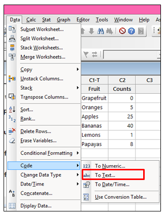
Using the Code Command
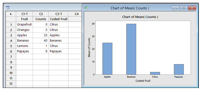
When working with text data, it is sometimes useful to reduce the number of categories by combining some of the categories into fewer groups. Consider the example below, where we have low or 0 counts for some of the citrus fruits:
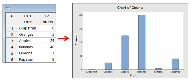
Rather than generating a bar chart with no bar for Grapefruit, we could combine some of the citrus fruits into a single Citrus category instead of listing them separately. The Code command in Minitab’s Data menu can help:
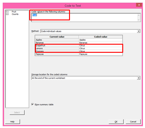
By coding our existing text values for Grapefruit, Oranges and Lemons to a new Text category called Citrus, we can reduce the number of categories. To do that in Minitab, we enter the original column listing the types of fruit in the first field. Then we change the values under Coded value from the current values (Lemons, Oranges, and Grapefruit) to their new value Citrus:
As a final step, we can tell Minitab where we’d like to store the coded results by using the Storage location for the coded columns drop-down list:
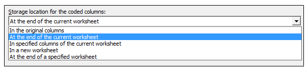
For this example, we’ll just keep the default and store the results at the end of the current worksheet and click OK. The coded results can easily be used to create a new bar chart that shows only the Citrus category instead of the individual fruits:
Using Conditional Formatting
This is a relatively new feature in Minitab, one which came about as the result of many requests from users who wanted the ability to control the appearance of the data in the worksheet. Because there are many options available in the new menu, we’ll just focus on two options as examples. The other options behave in a similar way, so a basic understanding of these two examples should be helpful in applying the other options in Conditional Formatting.
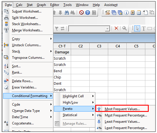
Often, raw text data is used to create Pareto charts to see the defects are most frequently occurring. But what if we want to highlight the most frequently occurring defect in the worksheet? We use Data > Conditional Formatting > Pareto > Most Frequent Values:
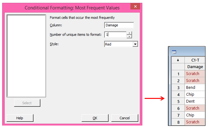
We enter our column listing the defects in the first field, and in the second field we can tell Minitab the number of unique items to highlight. For example, if we want to highlight the two most frequently listed defects, we enter 2. In this example, we only want to highlight the most common defect so we enter 1. Finally, we can tell Minitab what color we’d like to apply to the cells that meet our condition, and then we click OK to see the highlighted cells in the worksheet:
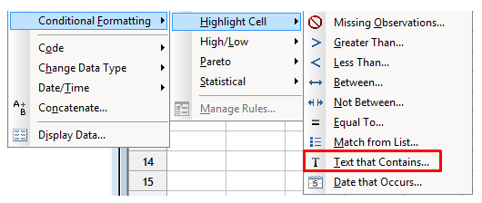
In some situations, it may be useful to highlight specific values in a text column. In fact, we may want multiple colors in a single column, each representing a specific category. For this situation we can use Conditional Formatting > Highlight Cell > Text that Contains:
With this option, we can tell Minitab the color we want for a cell that contains the text that we type into the Format cells that contain field:
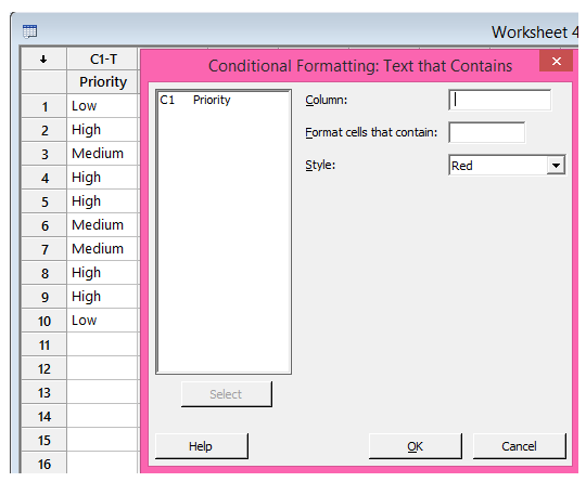
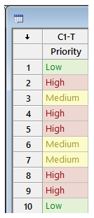
First we enter the column with the data in the first field, type the text we want to highlight in the second field (NOTE: This is case-sensitive), and then choose the color from the Style drop-down list. We can repeat this process if we want to apply multiple colors to a single column. In this example, the Low values will be shown in Green, the Medium values will be marked in Green, and the High values will be highlighted in Red:
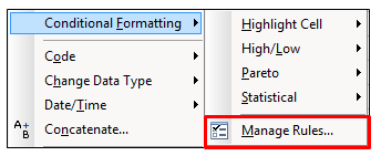
Finally, after applying conditional formatting to our worksheet, we’ll need an easy way to see all the rules we’ve applied and the ability to remove or change those rules. The Conditional Formatting menu’s Manage Rules option can make the magic happen:
The rules for each column are listed separately, so we choose a column to see the rules that have been applied by selecting the column from the drop-down list at the top:
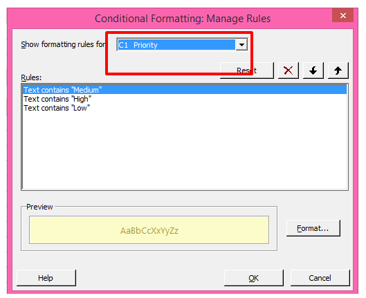
The rules applied to the selected column are listed under Rules. We can remove a specific rule by clicking on a rule in the Rules list, and then clicking the button with the red X.
We can also use the Format button to change the formatting of a specific rule. For example, I may want to change the rule for Medium from Yellow to my favorite color:
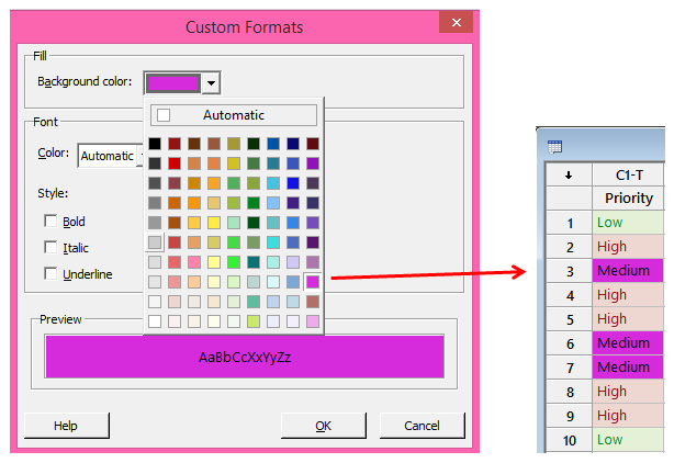
It’s much nicer in hot pink, wouldn’t you agree?
In my final post in this series, we’ll look at the new features that ease the pain of manipulating text data using the Editor menu.