How to Calculate BX Life, Part 2b: Handling Triangular Matrix Data

I thought 3 posts would capture all the thoughts I had about B10 Life. That is, until this question appeared on the Minitab LinkedIn group:

In case you missed it, my first post, How to Calculate B10 Life with Statistical Software, explains what B10 life is and how Minitab calculates this value. My second post, How to Calculate BX Life, Part 2, shows how to compute any BX life in Minitab. But before I round out my BX life blog series with rationale for why BX life is one of the best measures for reliability, I thought I’d take this opportunity to address the LinkedIn question—as you might wonder the same thing.

B10 Life and Warranty Analysis

BX Life can be a useful metric for establishing warranty periods for products. Why? Because it indicates the time at which X% of items in a population will fail. So a manufacturer might set a warranty period after a product’s B10 life, for instance, with the goal of minimizing the number of customers who will take advantage of the warranty should the product they purchase fail within the warranty period. Naturally, someone doing warranty analysis in Minitab should want to compute this value too! But looking at raw reliability field data, which are recorded in the form of a triangular matrix, it’s not obvious how to compute B10 life!

Warranty Input in Triangular Matrices

It’s common to keep track of reliability field data in the form of number of items shipped and number of items returned from a particular shipment over time. And when several shipments are made at different dates and their corresponding returns noted, the recorded data are in the form of a triangular matrix.

Minitab has a tool that helps you convert shipping and warranty return data from matrix form into a standard reliability data form of failures. 

Convert your data from a matrix form for easy analysis!

To demonstrate, let’s start with a new example and new data. If you’d like to follow along, navigate to our Online Help and select the Compressor.MTW file.

Here is what the data looks like:

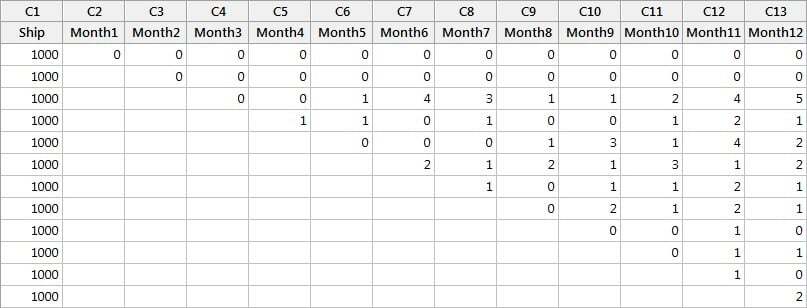
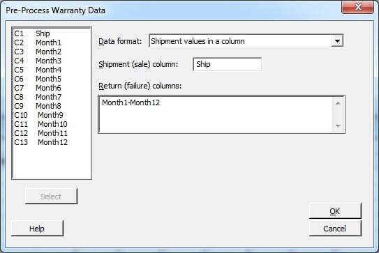
From here, you can use Minitab’s Pre-Process Warranty Data to reshape your data from triangular matrix format into interval censoring format. Select Stat > Reliability/Survival > Warranty Analysis > Pre-Process Warranty Data. For “Shipment (sale) column,” enter Ship. For “Return (failure) columns,” enter Month1-Month12. Click OK.

The Pre-Process step creates Start time, End time, and Frequencies columns in your worksheet! 

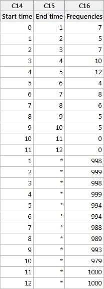
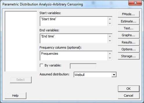
You can now use these columns to obtain BX life using Stat > Reliability/Survival > Distribution Analysis (Arbitrary Censoring) > Parametric Distribution Analysis. Enter Start time in “Start variables,” End time in “End variables,” and Frequencies in “Frequency columns (optional).” Also, make sure you have the appropriate assumed distribution selected. We’ll assume the Weibull distribution fits our data.

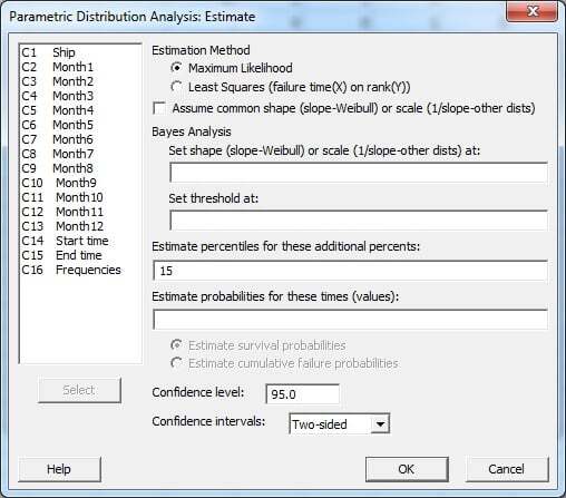
Click the Estimate button to enter percents to be estimated in addition to what’s provided in the default output (In our case, let’s ask for B15 Life—so enter a 15 in “Estimate percentiles for these additional percents”). 

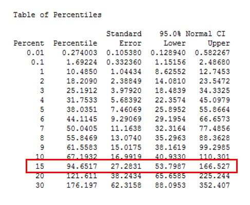
When we OK out of these dialogs, Minitab performs the analysis. Among the output Minitab provides is our handy Table of Percentiles, including our value for B15 life—or the time at which 15% of the items in our population will fail.

And there you have it!

Collecting warranty data and doing warranty analysis in Minitab shouldn’t prevent you from using reliability tools and metrics, such as BX life. In fact, letting Minitab reshape your data through the Pre-Process Warranty Data tool only makes your life easier when you dive into your reliability analysis!

Now, I promise, we’re well on our way to rounding out this series of posts, and in my next installment we'll look at the reasons BX life is a good metric to have in your reliability tool belt.

Case study:
Time-to-Market and Design for Reliability at the Speed of Light in Signify

Get ready for a light bulb moment! In a fast-changing industry where time-to-market and product reliability give a competitive edge, discover how the world’s leading lighting company Signify, rapidly validates new innovations. In this one hour webinar, Prof W.D. van Driel and Dr P. Watté will shed a light on design for reliability (DfR) using Minitab Statistical Software at Signify, the former Philips Lighting. Learn from real-life examples their methods to lower your development costs, improve your designs’ performance and compliance, and accelerate the testing of product design reliability. If you develop products intended to meet high specifications for years to come, you will discover how to reduce the risks and consequences of product failure and costly claims - for you and your customers.