


Ever use dental floss to cut soft cheese? Or Alka Seltzer to clean your toilet bowl? You can find a host of nonconventional uses for ordinary objects online. Some are more peculiar than others.
Ever use ordinary linear regression to evaluate a response (outcome) variable of counts?
Technically, ordinary linear regression was designed to evaluate a a continuous response variable. A continuous response variable, such as temperature or length, is measured along a continuous scale that includes fractional (decimal) values. In practice, however, ordinary linear regression is often used to evaluate a response of count data, which are whole numbers as 0, 1, 2, and so on.
You can do that. Just like you can use a banana to clean a DVD. But there are things to watch out for if you do that. To examine issues related to performing ordinary linear regression analysis with count data, consider the following scenario.
Kids, Ants, and Sandwiches
A bored kid in a backyard makes a great scientist. One day, three Australian kids wondered which of their lunch sandwiches would attract more meat ants: Peanut butter, Vegemite, or Ham and pickles.
Note: Meat ants are an aggressive species of Australian ant that can kill a poisonous cane toad. Vegemite is a slightly bitter, salty brown paste made from brewer’s yeast extract.
To test their hypotheses, the kids starting dropping pieces of the three sandwiches and counting the number of ants on each sandwich after a set amount of time. Years later, as an adult, one of the kids replicated this childhood experiment with increased rigor. You can find the details of his modified experiment and the sample data it produced on the web site of the American Statistical Association.
Preparing the Data
To make the data and the results easier to interpret, I coded and sorted the original sample data set using the Code and Sort commands in Minitab's Data menu. If you want to see those data manipulation maneuvers, click here to open the project file in Minitab, then open the Report Pad to see the instructions. If you don't have a copy of Minitab, you can download a free 30-day trial version.
After coding and sorting, the combination of factor levels for each sandwich used for ant bait are easy to see in the worksheet, and the data values are arranged in the order that they were collected.
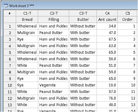
For example, row 9 shows that ham and pickles on rye with butter was the 9th piece of sandwich bait used—and it attracted 65 meat ants.
Performing Linear Regression
Are meat ants statistically more likely to swarm a ham sandwich—or will the pickles be a turnoff? Do they gravitate to the creamy comfort of butter? Or will salty, malty Vegemite drive them wild?
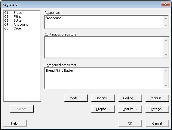
To evaluate the data using ordinary linear regression, choose Stat > Regression > Fit Regression Model. Fill out the dialog box as shown below and click OK.
First, examine the ANOVA table to determine whether any of the predictors are statistically significant.
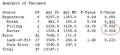
At the 0.1 level of significance, both Filling and Butter predictors are statistically significant (p-value < 0.1). What matters to a meat ant, it seems, is not the bread, but what's between it.
To see how each of the levels of the factors relate to the number of ants (the response), examine the Coefficients table.
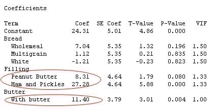
Each coefficient value is calculated in relation to the reference level for the variable, which has a coefficient of 0. Whatever level isn’t shown in the table is the reference level. So for the Filling variable, the reference level is Vegemite.
Tip: You can see the reference levels used for each variable by clicking the Coding button on the Regression dialog box. If you want the coefficients to be calculated relative to a different level, simply change the reference level in the drop-down list and rerun the analysis.
So what do these coefficient values mean? Generally speaking, larger coefficients are associated with a response of greater magnitude. The positive coefficients indicate a positive association, and the negative coefficients indicate a negative association.
For example, the positive coefficient of 27.28 for ham and pickles indicates that many more ants are attracted to the ham and pickles over Vegemite. The p-value of 0.000 for the coefficient indicates that the difference between ham and pickles and Vegemite is statistically significant. Based on these results, meat ants appear to be aptly named!
The Regression Equation: Caveat with a Count Response
The output for ordinary linear regression also includes a regression equation. The equation can be used to estimate the value of the response for specific values of the predictor variables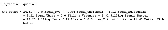
For categorical predictors, substitute a value of 1 into the equation for the levels at which you want to predict a response, and substitute 0 for the other levels.
For example, using the equation above, the number of meat ants that you can expect to be attracted by a peanut butter sandwich, without butter, on white bread, is estimated at: 24.31 + 7.04(0) + 1.12(0) - 1.21(1) + 0.0(0) + 8.31(1) + 27.28(0) + 0.0(1) + 11.40(0) ≈ 31.41 ants. (You can have Minitab do these calculations for you. Simply choose Stat > Regression > Regression > Predict and enter the predictor levels in the dialog box.)
One issue that can arise if you use ordinary linear regression with a count response is that, at certain predictor levels, the regression equation may estimate negative values for the response. But a negative "count" of ants—or anything else—doesn't make any sense. In that case, the equation may not be practically useful.
For this particular data set, it's not a problem. Using the regression equation, the lowest possible estimated response is for a Vegemite sandwich on white bread without butter (24.31 - 1.21), which yields an estimate of about 23 ants. Negative estimates don't occur primarily because the counts in this data set are all considerably greater than 0. But often that's not the case.
Evaluating the Model Fit and Assumptions
Regardless of whether you're performing ordinary linear regression with a continuous response variable or a discrete response variable of counts, it's important to assess the model fit, investigate extreme outliers, and check the model assumptions. If there's a serious problem, your results might not be valid.
The R-squared (adj) value suggests this model explains about half of the variation of the ant count (47.35%). Not great—but not not bad for a linear regression model with only a few categorical predictors. For this particular analysis, the ANOVA output also includes a p-value for lack-of-fit.

If the p-value for lack-of-fit is less than 0.05, there's statistically significant evidence that the model does not fit the data adequately. For this model, the p-value here is greater than 0.05. That means there's not sufficient evidence to conclude that the model doesn't fit well. That's a good thing.
Minitab's regression output also flags unusual observations, based on the size of their residuals. Residuals, also called "model errors", measure how much the response values estimated by the regression model differ from the actual response values in your data. The smaller a residual, the closer the value estimated by the model is to the actual value in your data. If a residual is unusually large, it suggests the the observation may be an outlier that's "bucking the trend" of your model.
For the ant count sample data, three observations are flagged as unusual:
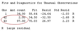
If you see unusual values in this table, it's not a cause for alarm. Generally, you can expect roughly 5% of the data values to have large standardized residuals. But if there's a lot more than that, or if the size of a residual is unusually large, you should investigate.
For this sample data set of 48 observations, the number of unusual observations is not worrisome. However, two of the observations (circled in red) appear to be very much out-of-whack with the other observations. To figure out why, I went back to the original sample data set online, and found this note from the experimenter:
"Two results are large outliers. A reading of 97 was due to…leaving a portion of sandwich behind from the previous observation (i.e., there were already ants there); and one of 2 was due to [the sandwich portion be placed] too far away from the entrance to the [ant] hill.”
Because these outliers can be attributed to a special (out-of-the-ordinary) cause, it would be OK to remove them and re-run the analysis, as long you clearly state that you have done so (and why). However, in this case, removing these two outliers doesn't significantly change the overall results of the linear regression analysis, anyway (for brevity, I won't include those results here).
Finally, examine the model assumptions for the regression analysis. In Minitab, choose Stat > Regression > Fit Regression Model. Then click Graphs and check Four in one.
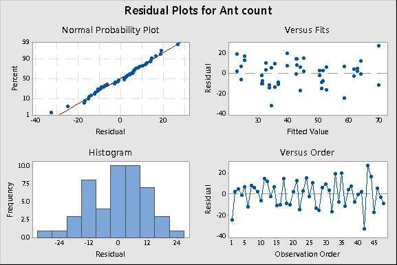
The two plots on the left (the Normal Probability Plot and the Histogram) help you assess whether the residuals are normally distributed. Although normality of the residuals is a formal assumption for ordinary linear regression, the analysis is fairly robust (resilient) to this assumption if the data set is sufficiently large (greater than 15 or so). Here, the points fall along the line of the normal probability plot and the histogram shows a fairly normal distribution. All is well..
Constant variance of the residuals is a more critical assumption for linear regression. That means the residuals should be distributed fairly evenly and randomly across all the fitted (estimated) values. To assess constant variance, look at the Residuals versus Fits plot in the upper right. In the plot above, the points appear to be randomly scattered on both sides of the line representing a residual value of 0. Again, no evidence of a problem.
With this sample data, using ordinary linear regression with a count response seems to work OK. But with different count data, might things have worked out differently? We'll examine that in the next post (Part 2).
Meanwhile, kick back and fix yourself a ham and pickle sandwich on rye with butter. And keep an eye out for meat ants.