How to Save a Failing Regression with PLS

Face it, you love regression analysis as much as I do. Regression is one of the most satisfying analyses in Minitab: get some predictors that should have a relationship to a response, go through a model selection process, interpret fit statistics like adjusted R² and predicted R², and make predictions. Yes, regression really is quite wonderful.

Except when it’s not. Dark, seedy corners of the data world exist, lying in wait to make regression confusing or impossible. Good old ordinary least squares regression, to be specific.

For instance, sometimes you have a lot of detail in your data, but not a lot of data. Want to see what I mean?

1. In Minitab, choose Help > Sample Data...
2. Open Soybean.mtw.

The data has 88 variables about soybeans, the results of near-infrared (NIR) spectroscopy at different wavelengths. But the data contains only 60 measurements, and the data are arranged to save 6 measurements for validation runs.

A Limit on Coefficients

With ordinary least squares regression, you only estimate as many coefficients as the data have samples. Thus, the traditional method that’s satisfactory in most cases would only let you estimate 53 coefficients for variables plus a constant coefficient.

This could leave you wondering about whether any of the other possible terms might have information that you need.

Multicollinearity

The NIR measurements are also highly collinear with each other. This multicollinearity complicates using statistical significance to choose among the variables to include in the model.

When the data have more variables than samples, especially when the predictor variables are highly collinear, it’s a good time to consider partial least squares regression.

How to Perform Partial Least Squares Regression

Try these steps if you want to follow along in Minitab Statistical Software using the soybean data:

1. Choose Stat > Regression > Partial Least Squares.
2. In Responses, enter Fat.
3. In Model, enter ‘1’-‘88’.
4. Click Options.
5. Under Cross-Validation, select Leave-one-out. Click OK.
6. Click Results.
7. Check Coefficients. Click OK twice.

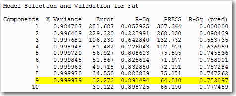
One of the great things about partial least squares regression is that it forms components and then does ordinary least squares regression with them. Thus the results include statistics that are familiar. For example, predicted R² is the criterion that Minitab uses to choose the number of components.

Each of the 9 components in the model that maximizes the predicted R² value is a complex linear combination of all 88 of the variables. So although the ANOVA table shows that you’re using only 9 degrees of freedom for the regression, the analysis uses information from all of the data.

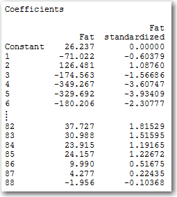
 The full list of standardized coefficients shows the relative importance of each predictor in the model. (I’m only showing a portion here because the table is 88 rows long.)

Ordinary least squares regression is a great tool that’s allowed people to make lots of good decision over the years. But there are times when it’s not satisfying. Got too much detail in your data? Partial least squares regression could be the answer.

Want more partial least squares regression now? Check out how Unifi used partial least squares to improve their processes faster.

The image of the soybeans is by Tammy Green and is licensed for reuse under this Creative Commons License.