A Field Guide to Statistical Distributions

by Matthew Barsalou, guest blogger. 

The old saying “if it walks like a duck, quacks like a duck and looks like a duck, then it must be a duck” may be appropriate in bird watching; however, the same idea can’t be applied when observing a statistical distribution. The dedicated ornithologist is often armed with binoculars and a field guide to the local birds and this should be sufficient. A statologist (I just made the word up, feel free to use it) on the other hand, is ill-equipped for the visual identification of his or her targets.

Normal, Student's t, Chi-Square, and F Distributions

Notice the upper two distributions in figure 1. The normal distribution and student’s t distribution may appear similar. However, the standard normal distribution is calculated using n and student’s t distribution is calculated using n-1. This may appear to be a minor difference, but when n is small, student’s t distribution displays much more peakedness. Student’s t distribution approaches the normal distribution as the sample size increases, but it never truly matches the shape of the normal distribution.

Observe the Chi-square and F distribution in the lower half of figure 1. The shapes of the distributions can vary and even the most astute observer will not be able to differentiate between them by eye. Many distributions can be sneaky like that. It is a part of their nature that we must accept as we can’t change it.

Figure 1

Binomial, Hypergeometric, Poisson, and Laplace Distributions

Notice the distributions illustrated in figure 2. A bird watcher may suddenly encounter four birds sitting in a tree; a quick check of a reference book may help to determine that they are all of a different species. The same can’t always be said for statistical distributions. Observe the binomial distribution, hypergeometric distribution and Poisson distribution. We can’t even be sure the three are not the same distribution. If they are together with a Laplace distribution, an observer may conclude “one of these does not appear to be the same as the others.” But they are all different, which our eyes alone may fail to tell us.

Figure 2

Weibull, Cauchy, Loglogistic, and Logistic Distributions

Suppose we observe the four distributions in figure 3.What are they? Could you tell if they were not labeled? We must identify them correctly before we can do anything with them. One is a Weibull distribution, but all four could conceivably be various Weibull distributions. The shape of the Weibull distribution varies based upon the shape parameter (κ) and scale parameter (λ).The Weibull distribution is a useful, but potentially devious distribution that can be much like the double-barred finch, which may be mistaken for an owl upon first glance.

Figure 3

Attempting to visually identify a statistical distribution can be very risky. Many distributions such as the Chi-Square and F distribution change shape drastically based on the number of degrees of freedom. Figure 4 shows various shapes for the Chi-Square, F distribution and the Weibull distribution. Figure 4 also compares a standard normal distribution with a standard deviation of one to a t distribution with 27 degrees of freedom; notices how the shapes overlap to the point where it is no longer possible to tell the two distributions apart.

Although there is no definitive Field Guide to Statistical Distributions to guide us, there are formulas available to correctly identify statistical distributions. We can also use Minitab Statistical Software to identify our distribution.

Figure 4

Go to Stat > Quality Tools > Individual Distribution Identification... and enter the column containing the data and the subgroup size. The results can be observed in either the session window (figure 5) or the graphical outputs shown in figures 6 through 9.

In this case, we can conclude we are observing a 3-parameter Weibull distribution based on the p value of 0.364.

Figure 5

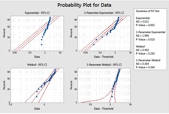Figure 6

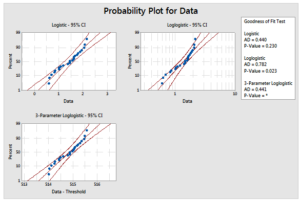Figure 7

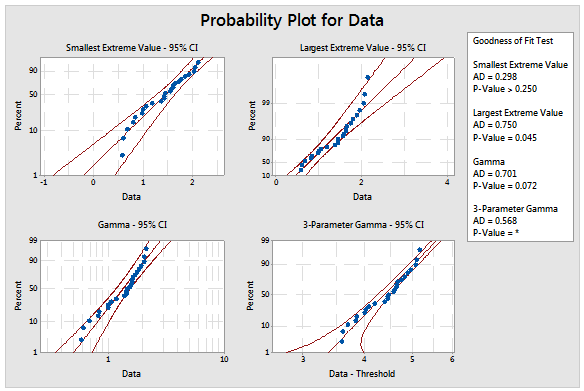Figure 8

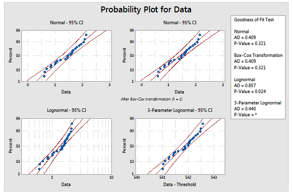Figure 9