


Transformations and non-normal distributions are typically the first approaches considered when the when the Normality test fails in a capability analysis. These approaches do not work when there are extreme outliers because they both assume the data come from a single common-cause variation distribution. But because extreme outliers typically represent special-cause variation, transformations and non-normal distributions are not good approaches for data that contain extreme outliers.
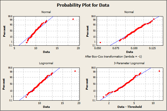
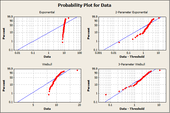
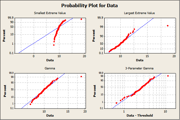
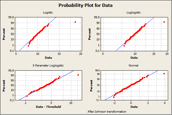
As an example, the four graphs below show distribution fits for a dataset with 99 values simulated from a N(m=10,s=1) distribution and 1 value simulated from a N(m=18,s=1) distribution. Two of the probability plots shown in these graphs assess the fit to a Normal Distribution after transforming the data. The remaining fourteen probability plots assess the fit to common (and some uncommon) non-normal distributions. None of the fits are adequate.
Method for Calculating Defect Rate
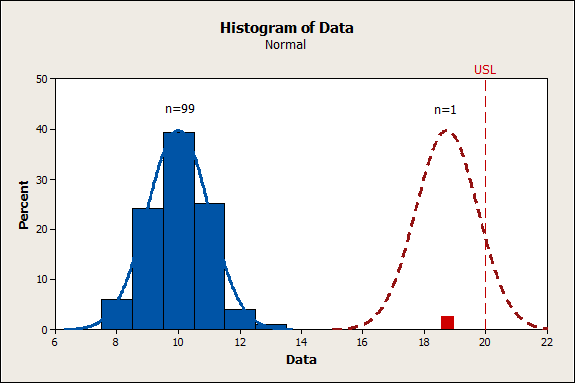
For process data with common cause variation that follows a Normal distribution, a reasonable approach for modeling extreme outliers is to assume the outliers represent a shift in the mean of the distribution, as shown in the next three graphs.
In most cases, there will not be enough data to measure the variation in the outlier distribution, so the variation in the outlier distribution will need to be assumed unchanged from the common cause distribution. This is consistent with the approach used in classic regression and ANOVA analyses, which assume a change in the mean does not affect the variation.
The defect rate can be estimated by using a weighted average of the defect rates from the common cause distribution and the outlier distribution. The weights come from the sample sizes for each distribution.
In the example below, this calculation would be as follows (POS = Probability of Out of Spec):
Defect Rate = [99*(POS Common Cause Dist.)+1*(POS Outlier Dist.)]/100
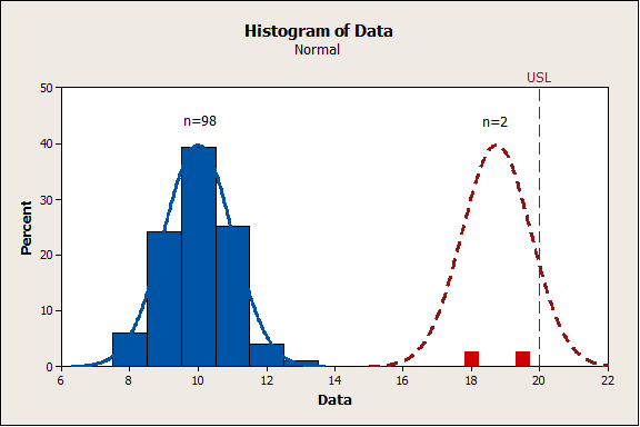
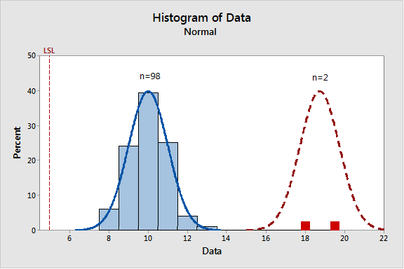
In the following two examples, this calculation would be as follows:
Defect Rate = [98*(POS Common Cause Dist.)+2*(POS Outlier Dist.)]/100
Important Considerations When Dealing with Extreme Outliers
It is critical to investigate extreme outliers and attempt to understand what caused them. The outlier(s) may be measurement errors or data entry errors, in which case they do not represent the true process and should appropriately adjusted.
If they are legitimate values, your number one priority should be to prevent future outliers from occurring and strive for process stability.
When you have special-cause variation in a capability analysis, you should not assume the defect rate estimated from the data represents the future defect rate of the process, no matter what approach you used. However, you may be able to get a rough estimate of the defect rate during the sampling period as long as the sample adequately represents the process during that time period.