


In regression, "sums of squares" are used to represent variation. In this post, we’ll use some sample data to walk through these calculations.
The sample data used in this post is available within Minitab by choosing Help > Sample Data , or File > Open Worksheet > Look in Minitab Sample Data folder (depending on your version of Minitab). The dataset is called ResearcherSalary.MTW , and contains data on salaries for researchers in a pharmaceutical company.
For this example we will use the data in C1, the salary, as Y or the response variable and C4, the years of experience as X or the predictor variable.
First, we can run our data through Minitab to see the results: Stat > Regression > Fitted Line Plot. The salary is the Y variable, and the years of experience is our X variable. The regression output will tell us about the relationship between years of experience and salary after we complete the dialog box as shown below, and then click OK:
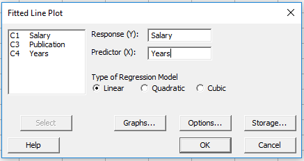
In the window above, I’ve also clicked the Storage button, selected the box next to Coefficients to store the coefficients from the regression equation in the worksheet. When we click OK in the window above, Minitab gives us two pieces of output:
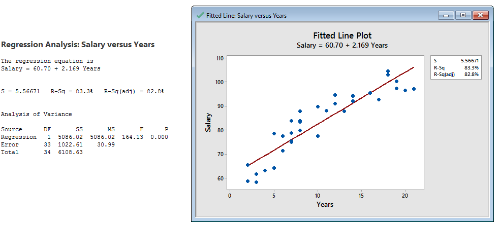
On the left side above we see the regression equation and the ANOVA (Analysis of Variance) table, and on the right side we see a graph that shows us the relationship between years of experience on the horizontal axis and salary on the vertical axis. Both the right and left side of the output above are conveying the same information. We can clearly see from the graph that as the years of experience increase, the salary increases, too (so years of experience and salary are positively correlated). For this post, we’ll focus on the SS (Sums of Squares) column in the Analysis of Variance table.
Calculating the Regression Sum of Squares
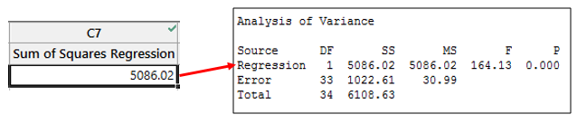
We see a SS value of 5086.02 in the Regression line of the ANOVA table above. That value represents the amount of variation in the salary that is attributable to the number of years of experience, based on this sample. Here's where that number comes from.
- Calculate the average response value (the salary). In Minitab, I’m using Stat > Basic Statistics > Store Descriptive Statistics:
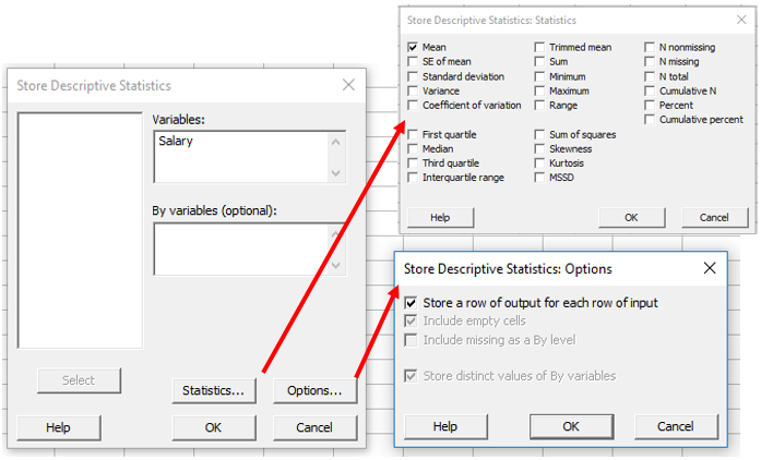
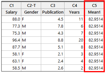
In addition to entering the Salary as the variable, I’ve clicked Statistics to make sure only Mean is selected, and I’ve also clicked Options and checked the box next to Store a row of output for each row of input. As a result, Minitab will store a value of 82.9514 (the average salary) in C5 35 times:
- Next, we will use the regression equation that Minitab gave us to calculate the fitted values. The fitted values are the salaries that our regression equation would predict, given the number of years of experience.
Our regression equation is Salary = 60.70 + 2.169*Years, so for every year of experience, we expect the salary to increase by 2.169.
The first row in the Years column in our sample data is 11, so if we use 11 in our equation we get 60.70 + 2.169*11 = 84.559. So with 11 years of experience our regression equation tells us the expected salary is about $84,000.
Rather than calculating this for every row in our worksheet manually, we can use Minitab’s calculator: Calc > Calculator (I used the stored coefficients in the worksheet to include more decimals in the regression equation that I’ve typed into the calculator):
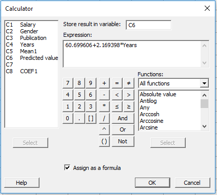
After clicking OK in the window above, Minitab will store the predicted salary value for every year in column C6. NOTE: In the regression graph we obtained, the red regression line represents the values we’ve just calculated in C6.
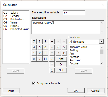
- Now that we have the average salary in C5 and the predicted values from our equation in C6, we can calculate the Sums of Squares for the Regression (the 5086.02). We’ll use Calc > Calculator again, and this time we will subtract the average salary from the predicted values, square those differences, and then add all of those squared differences together:
We square all the values because some of the predicted values from our equation are lower than the average, so those predicted values would be negative. If we sum together both positive and negative values, they will cancel each other out. But because we square the values, all observations will be taken into account.
We have just calculated the Sum of Squares for the regression by summing the squared values. Our results should match what we’d seen in the regression output previously:
Calculating the Error Sum of Squares
The Error Sum of Squares is the variation in the salary that is not explained by number of years of experience. For example, the additional variation in the salary could be due to the person’s gender, number of publications, or other variables that are not part of this model. Any variation that is not explained by the predictors in the model becomes part of the error term.
- To calculate the error sum of squares we will use the calculator (Calc > Calculator) again to subtract the fitted values (the salaries predicted by our regression equation) from the observed response (the actual salaries):
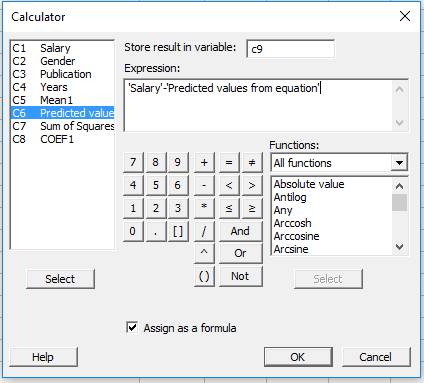
In C9, Minitab will store the differences between the actual salaries and what our equation predicted.
- Because we’re calculating sums of squares again, we’re going to square all the values we stored in C9, and then add them up to come up with the sum of squares for error:
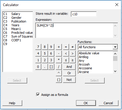
When we click OK in the calculator window above, we see that our calculated sum of squares for error matches Minitab’s output:
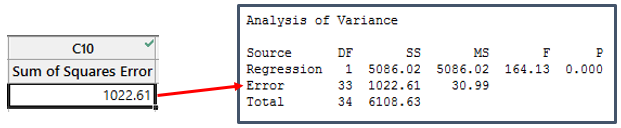
Finally the Sum of Squares total is calculated by adding the Regression and Error SS together: 5086.02 + 1022.61 = 6108.63.
I hope you’ve enjoyed this post, and that it helps demystify what sums of squares are. If you’d like to read more about regression, you may like some of Jim Frost’s regression tutorials.